Tutorial for MotrpacRatTraining6moData R package • MotrpacRatTraining6moData

Introduction

If you run into problems, please submit an issue here.

About this package

This package provides convenient access to the processed data and downstream analysis results presented in the main paper for the first large-scale multi-omic multi-tissue endurance exercise training study conducted in young adult rats by the Molecular Transducers of Physical Activity Consortium (MoTrPAC). Find the preprint on bioRxiv. We highly recommend skimming the preprint before using this package as it provides important context and much greater detail than we can provide here.

While the data in this package can be used by themselves, as demonstrated in this vignette, the MotrpacRatTraining6mo R package relies heavily on this package and provides many functions to help retrieve and explore the data. See the MotrpacRatTraining6mo vignette for examples.

About MoTrPAC

MoTrPAC is a national research consortium designed to discover and perform preliminary characterization of the range of molecular transducers (the “molecular map”) that underlie the effects of physical activity in humans. The program’s goal is to study the molecular changes that occur during and after exercise and ultimately to advance the understanding of how physical activity improves and preserves health. The six-year program is the largest targeted NIH investment of funds into the mechanisms of how physical activity improves health and prevents disease. See motrpac.org and motrpac-data.org for more details.

Installation

Install this package with devtools:

if (!require("devtools", quietly = TRUE)){
  install.packages("devtools")
}
options(timeout=1e5) # extend the timeout
devtools::install_github("MoTrPAC/MotrpacRatTraining6moData")

The output for a successful installation looks something like this. Note that the *** moving datasets to lazyload DB step takes the longest (~5 minutes):

Downloading GitHub repo MoTrPAC/MotrpacRatTraining6moData@HEAD
✓  checking for file ‘.../MoTrPAC-MotrpacRatTraining6moData-1c6478a/DESCRIPTION’ ...
─  preparing ‘MotrpacRatTraining6moData’:
✓  checking DESCRIPTION meta-information
─  checking for LF line-endings in source and make files and shell scripts
─  checking for empty or unneeded directories
─  building ‘MotrpacRatTraining6moData_1.3.2.tar.gz’ (1.3s)
   
* installing *source* package ‘MotrpacRatTraining6moData’ ...
** using staged installation
** R
** data
*** moving datasets to lazyload DB
** inst
** byte-compile and prepare package for lazy loading
** help
*** installing help indices
** building package indices
** testing if installed package can be loaded from temporary location
** testing if installed package can be loaded from final location
** testing if installed package keeps a record of temporary installation path
* DONE (MotrpacRatTraining6moData)

Troubleshooting

If you get this error after setting options(timeout=1e5):

Downloading GitHub repo MoTrPAC/MotrpacRatTraining6moData@HEAD
Error in utils::download.file(url, path, method = method, quiet = quiet,  : 
  download from 'https://api.github.com/repos/MoTrPAC/MotrpacRatTraining6moData/tarball/HEAD' failed
Error in `action()`:
! `class` is absent but must be supplied.
Run `rlang::last_error()` to see where the error occurred.

…this seems to be an intermittent issue seen only on Mac, not Linux or Windows. This was resolved by installing the newest version of R.

Last resort

If you can’t get devtools::install_github("MoTrPAC/MotrpacRatTraining6moData") to work, try this:

Go to https://api.github.com/repos/MoTrPAC/MotrpacRatTraining6moData/tarball/HEAD, which will automatically start downloading this repository in a tarball

Install the package from source:

install.packages("~/Downloads/MoTrPAC-MotrpacRatTraining6moData-0729e2e.tar.gz", 
  repos = NULL, 
  type = "source")
library(MotrpacRatTraining6moData)

Once we install this package, we can load the library.

library(MotrpacRatTraining6moData)
library(ggplot2) # for plots in this tutorial

Tip: To learn more about any data object, use ? to retrieve the documentation, e.g., ?METAB_FEATURE_ID_MAP. Note that MotrpacRatTraining6moData must be installed and loaded with library() for this to work.

Study design

Details of the experimental design can be found in the supplementary methods of the bioRxiv preprint. Briefly, 6-month-old young adult rats were subjected to progressive endurance exercise training for 1, 2, 4, or 8 weeks, with tissues collected 48 hours after the last training bout. Sex-matched sedentary, untrained rats were used as controls. Whole blood, plasma, and 18 solid tissues were analyzed using genomics, proteomics, metabolomics, and protein immunoassay technologies, with most assays performed in a subset of these tissues. Depending on the assay, between 3 and 6 replicates per sex per time point were analyzed.

Tissue and assay abbreviations

It is important to be aware of the tissue and assay abbreviations because they are used to name many data objects. The vectors of abbreviations are also available in TISSUE_ABBREV and ASSAY_ABBREV.

Tissues

ADRNL: adrenal gland
BAT: brown adipose tissue
BLOOD: whole blood
COLON: colon
CORTEX: cerebral cortex
HEART: heart
HIPPOC: hippocampus
HYPOTH: hypothalamus
KIDNEY: kidney
LIVER: liver
LUNG: lung
OVARY: ovaries (female gonads)
PLASMA: plasma from blood
SKM-GN: gastrocnemius (leg skeletal muscle)
SKM-VL: vastus lateralis (leg skeletal muscle)
SMLINT: small intestine
SPLEEN: spleen
TESTES: testes (male gonads)
VENACV: vena cava
WAT-SC: subcutaneous white adipose tissue

Assays/omes

ACETYL: acetylproteomics; protein site acetylation
ATAC: chromatin accessibility, ATAC-seq data
IMMUNO: multiplexed immunoassays (cytokines and hormones)
METAB: metabolomics and lipidomics
METHYL: DNA methylation, RRBS data
PHOSPHO: phosphoproteomics; protein site phosphorylation
PROT: global proteomics; protein abundance
TRNSCRPT: transcriptomics, RNA-Seq data
UBIQ: ubiquitylome; protein site ubiquitination

Summary of data

Here is a brief summary of the kinds of data included in this package:

Assay, tissue, sex, and training group abbreviations, codes, colors, and order used in plots
Phenotypic data, PHENO
Mapping between various feature identifiers, i.e., FEATURE_TO_GENE, RAT_TO_HUMAN_GENE
Ome-specific feature annotation, i.e., METAB_FEATURE_ID_MAP, METHYL_FEATURE_ANNOT (GCP only), ATAC_FEATURE_ANNOT (GCP only), PROT_FEATURE_ANNOT (GCP only), PHOSPHO_FEATURE_ANNOT (GCP only), UBIQ_FEATURE_ANNOT (GCP only), ACETYL_FEATURE_ANNOT (GCP only), TRNSCRPT_FEATURE_ANNOT (GCP only)
Ome-specific sample-level metadata, i.e., TRNSCRPT_META, ATAC_META, METHYL_META, IMMUNO_META, PHOSPHO_META, PROT_META, ACETYL_META, UBIQ_META
Raw counts for RNA-Seq (TRNSCRPT), ATAC-Seq (ATAC), and RRBS (METHYL) data, e.g., TRNSCRPT_LIVER_RAW_COUNTS. Note that epigenetic data (ATAC and METHYL) must be downloaded from Google Cloud Storage. See more details here.
Normalized sample-level data, e.g., TRNSCRPT_SKMGN_NORM_DATA
Differential analysis results, e.g., HEART_PROT_DA
Sample outliers excluded from differential analysis, OUTLIERS
Table of training-regulated features at 5% FDR, TRAINING_REGULATED_FEATURES
Bayesian graphical analysis inputs and results
Pathway enrichment of main graphical clusters, GRAPH_PW_ENRICH

A list of all the available data objects and a brief description are available here.

Principal component analysis

Here we show how to combine the normalized RNA-seq data from the gastrocnemius (leg skeletal muscle) with the phenotypic data to perform principal component analysis (PCA). We also take advantage of the training group colors.

# Load data 
# While this is not necessary, we want to make it clear what objects are available in the package.
# Note you can use data directly without loading with `data()`, e.g., `head(PHENO)`
data(PHENO) # phenotypic data
data(TRNSCRPT_SKMGN_NORM_DATA) # normalized gastrocnemius RNA-seq data
data(GROUP_COLORS) # hex colors for training groups 

# The first four columns in the sample-level data specify row meta-data; next columns are samples
# Note the "feature" column is only non-NA for training-regulated features at 5% FDR
TRNSCRPT_SKMGN_NORM_DATA[1:3,1:6]
#>   feature         feature_ID tissue    assay 90560015512 90581015512
#> 1    <NA> ENSRNOG00000000008 SKM-GN TRNSCRPT     0.04044    -0.09760
#> 2    <NA> ENSRNOG00000000012 SKM-GN TRNSCRPT     2.61487     2.78841
#> 3    <NA> ENSRNOG00000000021 SKM-GN TRNSCRPT     2.17049     1.70091
sample_ids = colnames(TRNSCRPT_SKMGN_NORM_DATA)[-c(1:4)]

# Perform PCA
skmgn_pca = stats::prcomp(t(TRNSCRPT_SKMGN_NORM_DATA[,sample_ids]))

# Make a data frame with some phenotypic data and the first 3 PCs
df = data.frame(
  group = PHENO[sample_ids,"group"],
  sex = PHENO[sample_ids,"sex"],
  skmgn_pca$x[,1:3] # take the first principal components
)

# Plot the first two PCs
ggplot(df, aes(x=PC1, y=PC2, colour=group, shape=sex)) + 
  geom_point(size=3)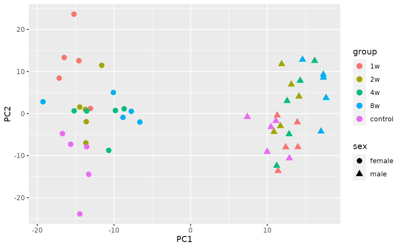


# Use GROUP_COLORS and make it prettier 
ggplot(df, aes(x=PC1, y=PC2, fill=group, shape=sex)) + 
  geom_point(size=3, colour="black") +
  scale_fill_manual(values=GROUP_COLORS) +
  scale_shape_manual(values=c(male=21, female=24)) +
  theme_bw() +
  guides(fill=guide_legend(override.aes = list(shape=21))) +
  labs(title="PCA of Gastrocnemius RNA-seq data") +
  theme(plot.title = element_text(hjust=0.5))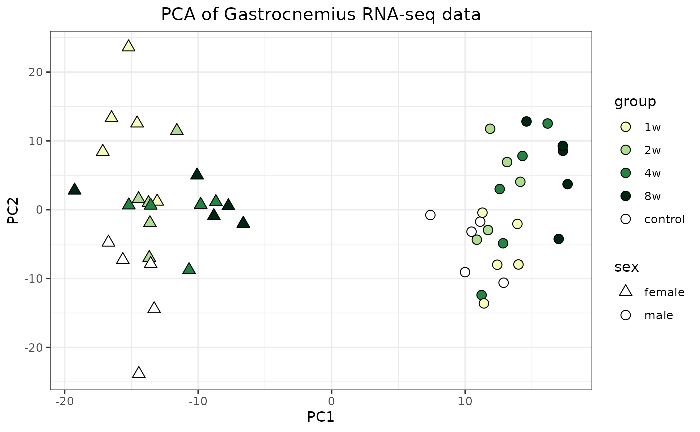

Compare RNA and protein data

Here we take the heart RNA-seq and global proteomics data, match their sample IDs, and map the features to gene IDs.

Data processing

First, load the normalized data from each ome.

rnaseq_d = TRNSCRPT_HEART_NORM_DATA
prot_d = PROT_HEART_NORM_DATA

By default, the column names of most sample-level data are vial labels, which are sample-specific identifiers. Different samples from the sample animal were processed for different assays. Therefore, in order to map between samples from the same animal across assays, we need to map sample IDs to participant IDs (PIDs) or biospecimen IDs (BIDs). Here, we map vial labels (sample IDs) to BIDs because BIDs are conveniently a substring of the vial labels. PHENO can also be used to map between vial labels (viallabel), PID (pid), and BID (bid).

## Match sample ids
#' A helper function for getting a named vector that maps biospecimen ids to sample ids
#' The biospecimen id of each sample is the substring of the sample id.
map_sample_to_bid = function(x){
  names(x) = substring(first=1, last=5, x)
  x
}
rnaseq_bid = map_sample_to_bid(colnames(rnaseq_d)[-c(1:4)])
prot_bid = map_sample_to_bid(colnames(prot_d)[-c(1:4)])
shared_bids = intersect(names(rnaseq_bid),names(prot_bid))

Now we used the FEATURE_TO_GENE map to map RNA-seq and proteomics feature IDs to gene symbols. FEATURE_TO_GENE is very large (>4M rows), so we start by subsetting it to the features in the current analysis.

dim(FEATURE_TO_GENE)
#> [1] 4044034       9
f2g = FEATURE_TO_GENE[
  FEATURE_TO_GENE$feature_ID %in% union(rnaseq_d$feature_ID,prot_d$feature_ID),
]
dim(f2g)
#> [1] 24591     9

Use the sample-to-BID mapping and the feature-to-gene mapping to subset the RNA-seq and proteomics data to overlapping BIDs and genes. For cases where multiple feature IDs map to the same gene, take the average value per BID.

# Get new RNA-seq and proteomics data frames
# here we compute the gene-wise average profiles, while limiting the
# data to the shared biospecimen ids
rnaseq_x = merge(rnaseq_d, f2g[,c("feature_ID","gene_symbol")], by="feature_ID")
rnaseq_x = stats::aggregate(
  rnaseq_x[,rnaseq_bid[shared_bids]], # get the shared samples
  by = list(rnaseq_x$gene_symbol), mean, na.rm=T)

# Same for proteomics
prot_x = merge(prot_d,f2g[,c("feature_ID","gene_symbol")],by="feature_ID")
prot_x = stats::aggregate(
  prot_x[,prot_bid[shared_bids]], # get the shared samples
  by = list(prot_x$gene_symbol),mean,na.rm=T)

# remove proteomics genes with missing values
prot_x = prot_x[!apply(is.na(prot_x),1,any),]

# Subset the data to the shared genes
rownames(rnaseq_x) = rnaseq_x[,1]
rnaseq_x = rnaseq_x[,-1]
rownames(prot_x) = prot_x[,1]
prot_x = prot_x[,-1]
shared_genes = intersect(rownames(rnaseq_x),rownames(prot_x))
prot_x = prot_x[shared_genes,]
rnaseq_x = rnaseq_x[shared_genes,]

Differential abundance analysis

Now we can perform a simple differential analysis between the males trained for 8 weeks and the sedentary control males to identify genes that are regulated by training. We do this separately for RNA-seq and proteomics data. We use t-tests here for simplicity, but a more appropriate way to compute differential abundance is to use tools like limma and DESeq2. Fortunately, these more robust results are also available in this package!

# Perform simple t-tests
ttest_wrapper <- function(x, groups, group1, group2){
  x1 = x[groups==group1]
  x2 = x[groups==group2]
  tres = t.test(x1,x2)
  return(c(
    "logFC" = unname(tres$estimate[1]-tres$estimate[2]),
    "tscore" = unname(tres$statistic),
    "p_value" = tres$p.value
  ))
}

# Compute t-tests for week 8 in males
training_groups = paste(
  PHENO[colnames(rnaseq_x),"sex"],
  PHENO[colnames(rnaseq_x),"group"], sep=","
)
male_8w_rnaseq_ttests = apply(rnaseq_x,
                              1,
                              ttest_wrapper,
                              groups=training_groups,
                              group1="male,8w",
                              group2="male,control")
male_8w_prot_ttests = apply(prot_x,
                            1,
                            ttest_wrapper,
                            groups=training_groups,
                            group1="male,8w",
                            group2="male,control")

# As we observed in the paper, the differential analysis results are mildly correlated:
cor(male_8w_rnaseq_ttests["tscore",], male_8w_prot_ttests["tscore",])
#> [1] 0.1920838

Compare to published results

Now we compare the results from the simple t-test above to the differential analysis results from DESeq2 (for RNA-seq) and limma (for proteomics).

rnaseq_DA = TRNSCRPT_HEART_DA
prot_DA = PROT_HEART_DA

# subset the results to 8w, males
rnaseq_DA = rnaseq_DA[rnaseq_DA$sex == "male" & rnaseq_DA$comparison_group=="8w",]
prot_DA = prot_DA[prot_DA$sex == "male" & prot_DA$comparison_group=="8w",]

# Add gene symbols
rnaseq_DA = merge(rnaseq_DA, f2g[,c("feature_ID","gene_symbol")], by="feature_ID")
prot_DA = merge(prot_DA, f2g[,c("feature_ID","gene_symbol")], by="feature_ID")

# Get the best t-test results per gene
get_best_zscore = function(zs){
  return(zs[abs(zs)==max(abs(zs),na.rm = T)][1])
}
rnaseq_t = tapply(rnaseq_DA$zscore,
                  rnaseq_DA$gene_symbol,
                  get_best_zscore)
prot_t = tapply(prot_DA$tscore,
                prot_DA$gene_symbol,
                get_best_zscore)

# Again, we see mild but non-zero correlation
cor(rnaseq_t[shared_genes],prot_t[shared_genes])
#> [1] 0.2126466

# Here we show an almost perfect correlation between the pre-computed 
# RNA-seq DESeq2 results and the simple t-tests performed above
plot(rnaseq_t[shared_genes],
     male_8w_rnaseq_ttests["tscore",shared_genes],
     main = "Transcriptomics DA, males at week 8",
     xlab = "DESeq2 t-score",ylab = "Simple t-test statistic",
     pch=20,col="gray");abline(0,1,lty=2)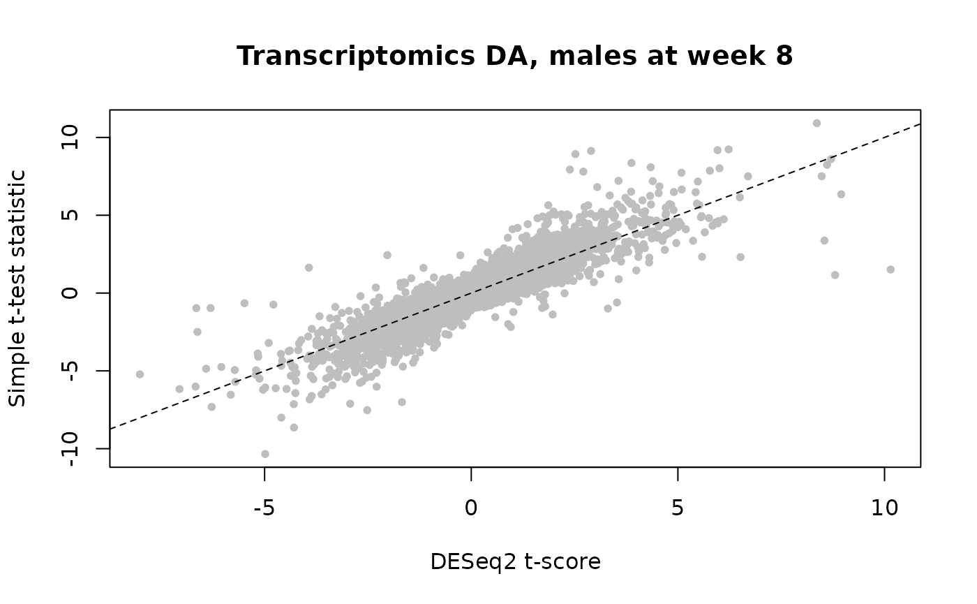


# Same as above, but for proteomics
plot(prot_t[shared_genes],male_8w_prot_ttests["tscore",shared_genes],
     main = "Proteomics DA, males at week 8",
     xlab = "limma t-score",ylab = "Simple t-test statistic",
     pch=20,col="gray");abline(0,1,lty=2)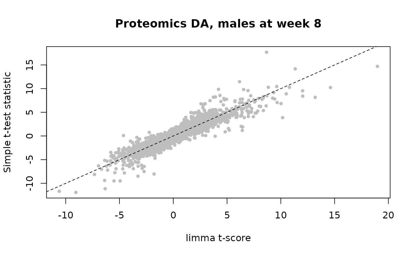

Getting help

For questions, bug reporting, and data requests for this package, please submit a new issue and include as many details as possible.

If the concern is related to functions provided in the MotrpacRatTraining6mo package, please submit an issue here instead.

Acknowledgements

MoTrPAC is supported by the National Institutes of Health (NIH) Common Fund through cooperative agreements managed by the National Institute of Diabetes and Digestive and Kidney Diseases (NIDDK), National Institute of Arthritis and Musculoskeletal Diseases (NIAMS), and National Institute on Aging (NIA).

Session Info

sessionInfo()
#> R version 4.3.2 (2023-10-31)
#> Platform: x86_64-pc-linux-gnu (64-bit)
#> Running under: Ubuntu 22.04.3 LTS
#> 
#> Matrix products: default
#> BLAS:   /usr/lib/x86_64-linux-gnu/openblas-pthread/libblas.so.3 
#> LAPACK: /usr/lib/x86_64-linux-gnu/openblas-pthread/libopenblasp-r0.3.20.so;  LAPACK version 3.10.0
#> 
#> locale:
#>  [1] LC_CTYPE=C.UTF-8       LC_NUMERIC=C           LC_TIME=C.UTF-8       
#>  [4] LC_COLLATE=C.UTF-8     LC_MONETARY=C.UTF-8    LC_MESSAGES=C.UTF-8   
#>  [7] LC_PAPER=C.UTF-8       LC_NAME=C              LC_ADDRESS=C          
#> [10] LC_TELEPHONE=C         LC_MEASUREMENT=C.UTF-8 LC_IDENTIFICATION=C   
#> 
#> time zone: UTC
#> tzcode source: system (glibc)
#> 
#> attached base packages:
#> [1] stats     graphics  grDevices utils     datasets  methods   base     
#> 
#> other attached packages:
#> [1] ggplot2_3.4.4                   MotrpacRatTraining6moData_2.0.0
#> 
#> loaded via a namespace (and not attached):
#>  [1] gtable_0.3.4      jsonlite_1.8.7    highr_0.10        dplyr_1.1.3      
#>  [5] compiler_4.3.2    tidyselect_1.2.0  stringr_1.5.0     jquerylib_0.1.4  
#>  [9] systemfonts_1.0.5 scales_1.2.1      textshaping_0.3.7 yaml_2.3.7       
#> [13] fastmap_1.1.1     R6_2.5.1          labeling_0.4.3    generics_0.1.3   
#> [17] knitr_1.45        tibble_3.2.1      desc_1.4.2        munsell_0.5.0    
#> [21] rprojroot_2.0.4   bslib_0.5.1       pillar_1.9.0      rlang_1.1.2      
#> [25] utf8_1.2.4        cachem_1.0.8      stringi_1.7.12    xfun_0.41        
#> [29] fs_1.6.3          sass_0.4.7        memoise_2.0.1     cli_3.6.1        
#> [33] withr_2.5.2       pkgdown_2.0.7     magrittr_2.0.3    digest_0.6.33    
#> [37] grid_4.3.2        lifecycle_1.0.4   vctrs_0.6.4       evaluate_0.23    
#> [41] glue_1.6.2        farver_2.1.1      ragg_1.2.6        fansi_1.0.5      
#> [45] colorspace_2.1-0  rmarkdown_2.25    purrr_1.0.2       pkgconfig_2.0.3  
#> [49] tools_4.3.2       htmltools_0.5.7