Tutorial for MotrpacRatTraining6mo R package

Introduction

If you run into problems, please submit an issue here.

About this package

This package provides functions to fetch, explore, and reproduce the processed data and downstream analysis results presented in the main paper for the first large-scale multi-omic multi-tissue endurance exercise training study conducted in young adult rats by the Molecular Transducers of Physical Activity Consortium (MoTrPAC). See our publication in Nature. We highly recommend skimming the paper before using this package as it provides important context and much greater detail than we can provide here.

While some of the functions in this package can be used by themselves, they were primarily written to analyze data in the MotrpacRatTraining6moData R package. See examples of how these data can be analyzed without this package in the MotrpacRatTraining6moData vignette.

About MoTrPAC

MoTrPAC is a national research consortium designed to discover and perform preliminary characterization of the range of molecular transducers (the “molecular map”) that underlie the effects of physical activity in humans. The program’s goal is to study the molecular changes that occur during and after exercise and ultimately to advance the understanding of how physical activity improves and preserves health. The six-year program is the largest targeted NIH investment of funds into the mechanisms of how physical activity improves health and prevents disease. See motrpac.org and motrpac-data.org for more details.

Setup

If you have not yet installed this R package, follow instructions here. Then load the library.

library(MotrpacRatTraining6mo)
#> Loading required package: MotrpacRatTraining6moData

As of v1.5.0, attaching MotrpacRatTraining6mo also attaches MotrpacRatTraining6moData, so an additional library(MotrpacRatTraining6moData) command is not necessary. For older versions of MotrpacRatTraining6mo, attach MotrpacRatTraining6moData directly. Attaching MotrpacRatTraining6moData makes it easier to load and look up documentation for data objects in the data package.

library(MotrpacRatTraining6moData)

We will also load several suggested packages, which are required to run some of the examples in this vignette.

suggests = c("gprofiler2","IHW","FELLA","foreach","KEGGREST","repfdr")
need_to_install = c()
for (p in suggests){
  if (!requireNamespace(p, quietly = TRUE)){
    need_to_install = c(need_to_install,p)
  }
}
if(length(need_to_install)>0){
  stop(sprintf("The following packages must be installed to run examples in this vignette:\n %s",
               paste(need_to_install, collapse=", ")))
}

Note: Data objects from the MotrpacRatTraining6moData package are indicated as variable names in all caps, e.g. PHENO, TRNSCRPT_LIVER_RAW_COUNTS.

Tip: To learn more about any data object or function, use ? to retrieve the documentation, e.g., ?METAB_FEATURE_ID_MAP, ?load_sample_data. Note that MotrpacRatTraining6mo must be installed and loaded with library() for this to work.

Study design

Details of the experimental design can be found in the supplementary information of our Nature publication. Briefly, 6-month-old young adult rats were subjected to progressive endurance exercise training for 1, 2, 4, or 8 weeks, with tissues collected 48 hours after the last training bout. Sex-matched sedentary, untrained rats were used as controls. Whole blood, plasma, and 18 solid tissues were analyzed using genomics, proteomics, metabolomics, and protein immunoassay technologies, with most assays performed in a subset of these tissues. Depending on the assay, between 3 and 6 replicates per sex per time point were analyzed.

Tissue and assay abbreviations

It is important to be aware of the tissue and assay abbreviations because they are used to name data objects and define arguments for many functions. The vectors of abbreviations are also available in TISSUE_ABBREV and ASSAY_ABBREV.

Tissues

ADRNL: adrenal gland
BAT: brown adipose tissue
BLOOD: whole blood
COLON: colon
CORTEX: cerebral cortex
HEART: heart
HIPPOC: hippocampus
HYPOTH: hypothalamus
KIDNEY: kidney
LIVER: liver
LUNG: lung
OVARY: ovaries (female gonads)
PLASMA: plasma from blood
SKM-GN: gastrocnemius (leg skeletal muscle)
SKM-VL: vastus lateralis (leg skeletal muscle)
SMLINT: small intestine
SPLEEN: spleen
TESTES: testes (male gonads)
VENACV: vena cava
WAT-SC: subcutaneous white adipose tissue

Assays/omes

ACETYL: acetylproteomics; protein site acetylation
ATAC: chromatin accessibility, ATAC-seq data
IMMUNO: multiplexed immunoassays (cytokines and hormones)
METAB: metabolomics and lipidomics
METHYL: DNA methylation, RRBS data
PHOSPHO: phosphoproteomics; protein site phosphorylation
PROT: global proteomics; protein abundance
TRNSCRPT: transcriptomics, RNA-Seq data
UBIQ: ubiquitylome; protein site ubiquitination

Data in MotrpacRatTraining6moData

While some of the functions in this package can be used by themselves, they were primarily written to analyze data in the MotrpacRatTraining6moData R package.

Here is a brief summary of the kinds of data included in MotrpacRatTraining6moData:

Assay, tissue, sex, and training group abbreviations, codes, colors, and order used in plots
Phenotypic data, PHENO
Mapping between various feature identifiers, i.e., FEATURE_TO_GENE, RAT_TO_HUMAN_GENE
Ome-specific feature annotation, i.e., METAB_FEATURE_ID_MAP, METHYL_FEATURE_ANNOT (GCP only), ATAC_FEATURE_ANNOT (GCP only)
Ome-specific sample-level metadata, i.e., TRNSCRPT_META, ATAC_META, METHYL_META, IMMUNO_META, PHOSPHO_META, PROT_META, ACETYL_META, UBIQ_META
Raw counts for RNA-Seq (TRNSCRPT), ATAC-Seq (ATAC), and RRBS (METHYL) data, e.g., TRNSCRPT_LIVER_RAW_COUNTS. Note that epigenetic data (ATAC and METHYL) must be downloaded from Google Cloud Storage.
Normalized sample-level data, e.g., TRNSCRPT_SKMGN_NORM_DATA
Differential analysis results, e.g., HEART_PROT_DA (see more details below)
Sample outliers excluded from differential analysis, OUTLIERS
Table of training-regulated features at 5% FDR, TRAINING_REGULATED_FEATURES
Bayesian graphical analysis inputs and results (see more details below)
Pathway enrichment of main graphical clusters, GRAPH_PW_ENRICH

For more details about the MotrpacRatTraining6moData R package, see its vignette. The remainder of this vignette will focus on functions available in MotrpacRatTraining6mo.

MotrpacRatTraining6mo includes several functions to easily fetch and compile data from MotrpacRatTraining6moData.

Use load_sample_data() to load sample-level data for a specific ome and tissue. Here we fetch various forms of the sample-level RNA-Seq (TRNSCRPT) data for brown adipose tissue (BAT) as an example.

# Load RNA-seq raw counts for brown adipose tissue 
data = load_sample_data("BAT", "TRNSCRPT", normalized = FALSE)

# Load the normalized RNA-seq data for brown adipose tissue instead
data = load_sample_data("BAT", "TRNSCRPT")

# Load the normalized RNA-seq data for brown adipose tissue, but exclude sample outliers 
data = load_sample_data("BAT", "TRNSCRPT", exclude_outliers = TRUE)

# Load the normalized RNA-seq data for brown adipose tissue for training-regulated features only
data = load_sample_data("BAT", "TRNSCRPT", training_regulated_only = TRUE)

load_sample_data() will tell you if the specified dataset doesn’t exist.

data = load_sample_data("VENACV", "PROT")
#> Warning in load_sample_data("VENACV", "PROT"): No data returned for tissue
#> VENACV and assay PROT with current arguments.

load_sample_data() will also download epigenetic data from Google Cloud Storage.

Note: Epigenetic data require substantially more memory than other omes.

# Load ATAC-seq raw counts for hippocampus, excluding outliers 
data = load_sample_data("HIPPOC", 
                        "ATAC", 
                        exclude_outliers = TRUE, 
                        normalized = FALSE, 
                        scratchdir = "/tmp")

We can plot the normalized sample-level data for a single feature using plot_feature_normalized_data(). All of the following examples are different ways to plot the same feature.

plot_feature_normalized_data(feature = "PROT;SKM-GN;NP_786937.1",
                             add_gene_symbol = TRUE)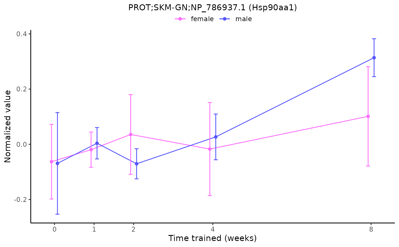


plot_feature_normalized_data(assay = "PROT",
                             tissue = "SKM-GN",
                             feature_ID = "NP_786937.1",
                             exclude_outliers = TRUE,
                             scale_x_by_time = FALSE)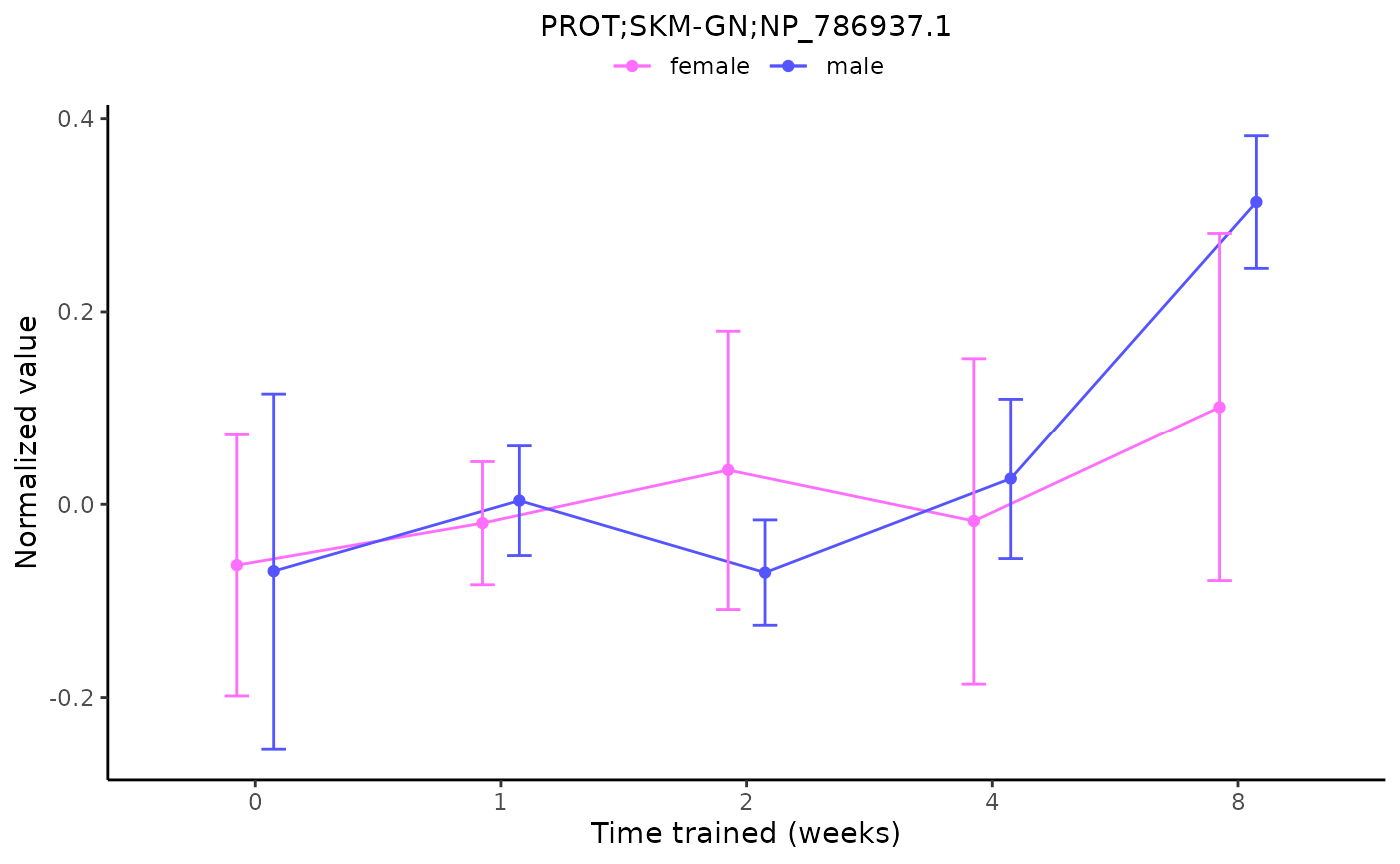


plot_feature_normalized_data(assay = "PROT",
                             tissue = "SKM-GN",
                             feature_ID = "NP_786937.1",
                             facet_by_sex = TRUE)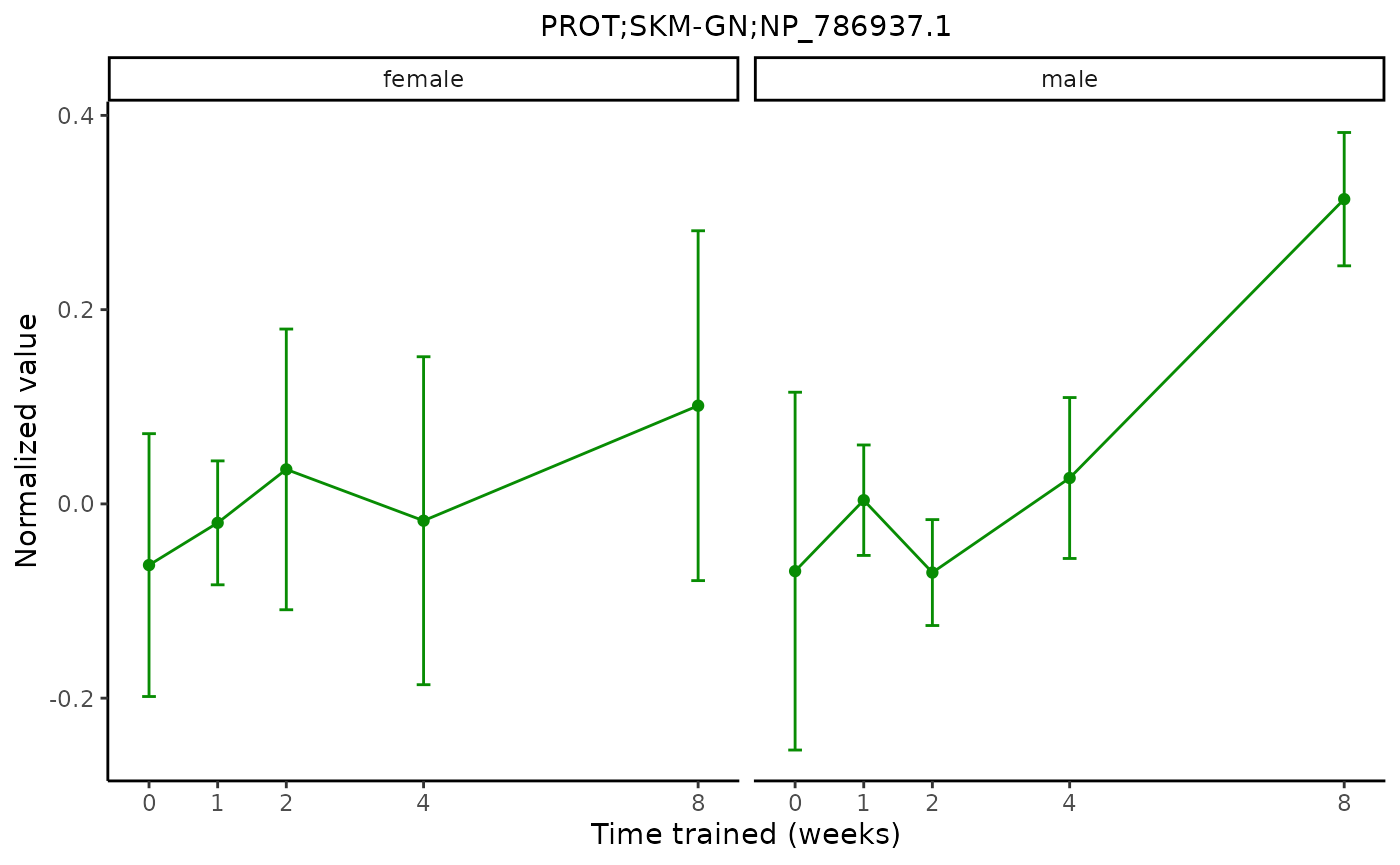

combine_normalized_data() is a wrapper for load_sample_data() that returns combined sample-level normalized data for multiple datasets. Note that the sample-specific vial labels used as column names for most of the sample-level data are replaced with rat-specific participant IDs (PIDs) to allow measurements from multiple datasets for the same animal to be concatenated.

# Return all normalized RNA-seq data
data = combine_normalized_data(assays = "TRNSCRPT")

# Return all normalized proteomics data. Exclude outliers 
data = combine_normalized_data(assays = c("PROT","UBIQ","PHOSPHO","ACETYL"),
                               exclude_outliers = TRUE)

# Return normalized ATAC-seq data for training-regulated features 
data = combine_normalized_data(assays = "ATAC", 
                               training_regulated_only = TRUE)

# Return all non-epigenetic data
# Note that the "include_epigen" argument is FALSE by default
data = combine_normalized_data()

Similarly, combine_da_results() concatenates differential analysis results for multiple datasets.

# Return all non-epigenetic differential analysis results, 
# including meta-regression results for metabolomics
res = combine_da_results()

# Return METHYL and ATAC differential analysis results for gastrocnemius 
res = combine_da_results(tissues="SKM-GN", 
                         assays=c("ATAC","METHYL"),
                         include_epigen=TRUE)

transcript_prep_data() and atac_prep_data() are functions used within the differential analysis functions for TRNSCRPT and ATAC data. They collect the filtered raw counts, normalized sample-level data, phenotypic data, and ome-specific sample metadata, covariates, and outliers associated with a given tissue.

A few additional functions are provided to fetch epigenetic data from Google Cloud Storage:

load_methyl_raw_data(): Return the unfiltered raw counts for a given tissue.
load_methyl_feature_annotation(): Return the METHYL feature annotation file.
load_atac_feature_annotation(): Return the ATAC feature annotation file.
get_rdata_from_url(): If you know the URL for a specific RData file in GCS, you can use this function to return the object using the url argument. Full URLs for all of the epigenetic data are available in the README for the MotrpacRatTraining6moData package.

Finally, list_available_data() returns a list of all of the available data objects in the specified package.

list_available_data("MotrpacRatTraining6moData")
#>   [1] "ACETYL_HEART_DA"                         
#>   [2] "ACETYL_HEART_NORM_DATA"                  
#>   [3] "ACETYL_LIVER_DA"                         
#>   [4] "ACETYL_LIVER_NORM_DATA"                  
#>   [5] "ACETYL_META"                             
#>   [6] "ASSAY_ABBREV"                            
#>   [7] "ASSAY_ABBREV_TO_CODE"                    
#>   [8] "ASSAY_CODE_TO_ABBREV"                    
#>   [9] "ASSAY_COLORS"                            
#>  [10] "ASSAY_ORDER"                             
#>  [11] "ATAC_BAT_NORM_DATA_05FDR"                
#>  [12] "ATAC_HEART_NORM_DATA_05FDR"              
#>  [13] "ATAC_HIPPOC_NORM_DATA_05FDR"             
#>  [14] "ATAC_KIDNEY_NORM_DATA_05FDR"             
#>  [15] "ATAC_LIVER_NORM_DATA_05FDR"              
#>  [16] "ATAC_LUNG_NORM_DATA_05FDR"               
#>  [17] "ATAC_META"                               
#>  [18] "ATAC_SKMGN_NORM_DATA_05FDR"              
#>  [19] "ATAC_WATSC_NORM_DATA_05FDR"              
#>  [20] "FEATURE_TO_GENE"                         
#>  [21] "FEATURE_TO_GENE_FILT"                    
#>  [22] "GENE_UNIVERSES"                          
#>  [23] "GRAPH_COMPONENTS"                        
#>  [24] "GRAPH_PW_ENRICH"                         
#>  [25] "GRAPH_STATES"                            
#>  [26] "GROUP_COLORS"                            
#>  [27] "IMMUNO_ADRNL_DA"                         
#>  [28] "IMMUNO_BAT_DA"                           
#>  [29] "IMMUNO_COLON_DA"                         
#>  [30] "IMMUNO_CORTEX_DA"                        
#>  [31] "IMMUNO_HEART_DA"                         
#>  [32] "IMMUNO_HIPPOC_DA"                        
#>  [33] "IMMUNO_KIDNEY_DA"                        
#>  [34] "IMMUNO_LIVER_DA"                         
#>  [35] "IMMUNO_LUNG_DA"                          
#>  [36] "IMMUNO_META"                             
#>  [37] "IMMUNO_NORM_DATA_FLAT"                   
#>  [38] "IMMUNO_NORM_DATA_NESTED"                 
#>  [39] "IMMUNO_OVARY_DA"                         
#>  [40] "IMMUNO_PLASMA_DA"                        
#>  [41] "IMMUNO_SKMGN_DA"                         
#>  [42] "IMMUNO_SKMVL_DA"                         
#>  [43] "IMMUNO_SMLINT_DA"                        
#>  [44] "IMMUNO_SPLEEN_DA"                        
#>  [45] "IMMUNO_TESTES_DA"                        
#>  [46] "IMMUNO_WATSC_DA"                         
#>  [47] "METAB_ADRNL_DA"                          
#>  [48] "METAB_ADRNL_DA_METAREG"                  
#>  [49] "METAB_BAT_DA"                            
#>  [50] "METAB_BAT_DA_METAREG"                    
#>  [51] "METAB_COLON_DA"                          
#>  [52] "METAB_COLON_DA_METAREG"                  
#>  [53] "METAB_CORTEX_DA"                         
#>  [54] "METAB_CORTEX_DA_METAREG"                 
#>  [55] "METAB_FEATURE_ID_MAP"                    
#>  [56] "METAB_HEART_DA"                          
#>  [57] "METAB_HEART_DA_METAREG"                  
#>  [58] "METAB_HIPPOC_DA"                         
#>  [59] "METAB_HIPPOC_DA_METAREG"                 
#>  [60] "METAB_HYPOTH_DA"                         
#>  [61] "METAB_HYPOTH_DA_METAREG"                 
#>  [62] "METAB_KIDNEY_DA"                         
#>  [63] "METAB_KIDNEY_DA_METAREG"                 
#>  [64] "METAB_LIVER_DA"                          
#>  [65] "METAB_LIVER_DA_METAREG"                  
#>  [66] "METAB_LUNG_DA"                           
#>  [67] "METAB_LUNG_DA_METAREG"                   
#>  [68] "METAB_NORM_DATA_FLAT"                    
#>  [69] "METAB_NORM_DATA_NESTED"                  
#>  [70] "METAB_OVARY_DA"                          
#>  [71] "METAB_OVARY_DA_METAREG"                  
#>  [72] "METAB_PLASMA_DA"                         
#>  [73] "METAB_PLASMA_DA_METAREG"                 
#>  [74] "METAB_SKMGN_DA"                          
#>  [75] "METAB_SKMGN_DA_METAREG"                  
#>  [76] "METAB_SKMVL_DA"                          
#>  [77] "METAB_SKMVL_DA_METAREG"                  
#>  [78] "METAB_SMLINT_DA"                         
#>  [79] "METAB_SMLINT_DA_METAREG"                 
#>  [80] "METAB_SPLEEN_DA"                         
#>  [81] "METAB_SPLEEN_DA_METAREG"                 
#>  [82] "METAB_TESTES_DA"                         
#>  [83] "METAB_TESTES_DA_METAREG"                 
#>  [84] "METAB_VENACV_DA"                         
#>  [85] "METAB_VENACV_DA_METAREG"                 
#>  [86] "METAB_WATSC_DA"                          
#>  [87] "METAB_WATSC_DA_METAREG"                  
#>  [88] "METHYL_BAT_NORM_DATA_05FDR"              
#>  [89] "METHYL_HEART_NORM_DATA_05FDR"            
#>  [90] "METHYL_HIPPOC_NORM_DATA_05FDR"           
#>  [91] "METHYL_KIDNEY_NORM_DATA_05FDR"           
#>  [92] "METHYL_LIVER_NORM_DATA_05FDR"            
#>  [93] "METHYL_LUNG_NORM_DATA_05FDR"             
#>  [94] "METHYL_META"                             
#>  [95] "METHYL_SKMGN_NORM_DATA_05FDR"            
#>  [96] "METHYL_WATSC_NORM_DATA_05FDR"            
#>  [97] "OUTLIERS"                                
#>  [98] "PATHWAY_PARENTS"                         
#>  [99] "PHENO"                                   
#> [100] "PHOSPHO_CORTEX_DA"                       
#> [101] "PHOSPHO_CORTEX_NORM_DATA"                
#> [102] "PHOSPHO_HEART_DA"                        
#> [103] "PHOSPHO_HEART_NORM_DATA"                 
#> [104] "PHOSPHO_KIDNEY_DA"                       
#> [105] "PHOSPHO_KIDNEY_NORM_DATA"                
#> [106] "PHOSPHO_LIVER_DA"                        
#> [107] "PHOSPHO_LIVER_NORM_DATA"                 
#> [108] "PHOSPHO_LUNG_DA"                         
#> [109] "PHOSPHO_LUNG_NORM_DATA"                  
#> [110] "PHOSPHO_META"                            
#> [111] "PHOSPHO_SKMGN_DA"                        
#> [112] "PHOSPHO_SKMGN_NORM_DATA"                 
#> [113] "PHOSPHO_WATSC_DA"                        
#> [114] "PHOSPHO_WATSC_NORM_DATA"                 
#> [115] "PROT_CORTEX_DA"                          
#> [116] "PROT_CORTEX_NORM_DATA"                   
#> [117] "PROT_HEART_DA"                           
#> [118] "PROT_HEART_NORM_DATA"                    
#> [119] "PROT_KIDNEY_DA"                          
#> [120] "PROT_KIDNEY_NORM_DATA"                   
#> [121] "PROT_LIVER_DA"                           
#> [122] "PROT_LIVER_NORM_DATA"                    
#> [123] "PROT_LUNG_DA"                            
#> [124] "PROT_LUNG_NORM_DATA"                     
#> [125] "PROT_META"                               
#> [126] "PROT_SKMGN_DA"                           
#> [127] "PROT_SKMGN_NORM_DATA"                    
#> [128] "PROT_WATSC_DA"                           
#> [129] "PROT_WATSC_NORM_DATA"                    
#> [130] "RAT_TO_HUMAN_GENE"                       
#> [131] "RAT_TO_HUMAN_PHOSPHO"                    
#> [132] "REPEATED_FEATURES"                       
#> [133] "REPFDR_INPUTS"                           
#> [134] "REPFDR_RES"                              
#> [135] "SEX_COLORS"                              
#> [136] "TISSUE_ABBREV"                           
#> [137] "TISSUE_ABBREV_TO_CODE"                   
#> [138] "TISSUE_CODE_TO_ABBREV"                   
#> [139] "TISSUE_COLORS"                           
#> [140] "TISSUE_ORDER"                            
#> [141] "TRAINING_REGULATED_FEATURES"             
#> [142] "TRAINING_REGULATED_NORM_DATA"            
#> [143] "TRAINING_REGULATED_NORM_DATA_NO_OUTLIERS"
#> [144] "TRNSCRPT_ADRNL_DA"                       
#> [145] "TRNSCRPT_ADRNL_NORM_DATA"                
#> [146] "TRNSCRPT_ADRNL_RAW_COUNTS"               
#> [147] "TRNSCRPT_BAT_DA"                         
#> [148] "TRNSCRPT_BAT_NORM_DATA"                  
#> [149] "TRNSCRPT_BAT_RAW_COUNTS"                 
#> [150] "TRNSCRPT_BLOOD_DA"                       
#> [151] "TRNSCRPT_BLOOD_NORM_DATA"                
#> [152] "TRNSCRPT_BLOOD_RAW_COUNTS"               
#> [153] "TRNSCRPT_COLON_DA"                       
#> [154] "TRNSCRPT_COLON_NORM_DATA"                
#> [155] "TRNSCRPT_COLON_RAW_COUNTS"               
#> [156] "TRNSCRPT_CORTEX_DA"                      
#> [157] "TRNSCRPT_CORTEX_NORM_DATA"               
#> [158] "TRNSCRPT_CORTEX_RAW_COUNTS"              
#> [159] "TRNSCRPT_HEART_DA"                       
#> [160] "TRNSCRPT_HEART_NORM_DATA"                
#> [161] "TRNSCRPT_HEART_RAW_COUNTS"               
#> [162] "TRNSCRPT_HIPPOC_DA"                      
#> [163] "TRNSCRPT_HIPPOC_NORM_DATA"               
#> [164] "TRNSCRPT_HIPPOC_RAW_COUNTS"              
#> [165] "TRNSCRPT_HYPOTH_DA"                      
#> [166] "TRNSCRPT_HYPOTH_NORM_DATA"               
#> [167] "TRNSCRPT_HYPOTH_RAW_COUNTS"              
#> [168] "TRNSCRPT_KIDNEY_DA"                      
#> [169] "TRNSCRPT_KIDNEY_NORM_DATA"               
#> [170] "TRNSCRPT_KIDNEY_RAW_COUNTS"              
#> [171] "TRNSCRPT_LIVER_DA"                       
#> [172] "TRNSCRPT_LIVER_NORM_DATA"                
#> [173] "TRNSCRPT_LIVER_RAW_COUNTS"               
#> [174] "TRNSCRPT_LUNG_DA"                        
#> [175] "TRNSCRPT_LUNG_NORM_DATA"                 
#> [176] "TRNSCRPT_LUNG_RAW_COUNTS"                
#> [177] "TRNSCRPT_META"                           
#> [178] "TRNSCRPT_OVARY_DA"                       
#> [179] "TRNSCRPT_OVARY_NORM_DATA"                
#> [180] "TRNSCRPT_OVARY_RAW_COUNTS"               
#> [181] "TRNSCRPT_SKMGN_DA"                       
#> [182] "TRNSCRPT_SKMGN_NORM_DATA"                
#> [183] "TRNSCRPT_SKMGN_RAW_COUNTS"               
#> [184] "TRNSCRPT_SKMVL_DA"                       
#> [185] "TRNSCRPT_SKMVL_NORM_DATA"                
#> [186] "TRNSCRPT_SKMVL_RAW_COUNTS"               
#> [187] "TRNSCRPT_SMLINT_DA"                      
#> [188] "TRNSCRPT_SMLINT_NORM_DATA"               
#> [189] "TRNSCRPT_SMLINT_RAW_COUNTS"              
#> [190] "TRNSCRPT_SPLEEN_DA"                      
#> [191] "TRNSCRPT_SPLEEN_NORM_DATA"               
#> [192] "TRNSCRPT_SPLEEN_RAW_COUNTS"              
#> [193] "TRNSCRPT_TESTES_DA"                      
#> [194] "TRNSCRPT_TESTES_NORM_DATA"               
#> [195] "TRNSCRPT_TESTES_RAW_COUNTS"              
#> [196] "TRNSCRPT_VENACV_DA"                      
#> [197] "TRNSCRPT_VENACV_NORM_DATA"               
#> [198] "TRNSCRPT_VENACV_RAW_COUNTS"              
#> [199] "TRNSCRPT_WATSC_DA"                       
#> [200] "TRNSCRPT_WATSC_NORM_DATA"                
#> [201] "TRNSCRPT_WATSC_RAW_COUNTS"               
#> [202] "UBIQ_HEART_DA"                           
#> [203] "UBIQ_HEART_NORM_DATA"                    
#> [204] "UBIQ_LIVER_DA"                           
#> [205] "UBIQ_LIVER_NORM_DATA"                    
#> [206] "UBIQ_META"

If the MotrpacRatTraining6moData library is attached, you can learn more about any of these data objects with ?, e.g., ?TISSUE_COLORS, and you can load data objects into your environment using data(), e.g., data(TRAINING_REGULATED_FEATURES).

Differential analysis

More details about the differential analysis methods are available in the supplementary information of our Nature publication. Simply put, the training differential analysis considers all training groups for each sex (sedentary controls and 4 training time points) to determine if the analyte significantly changes in either sex at any point during the training time course. The adjusted p-values from this analysis were used to determine the set of analytes that are regulated by endurance exercise training at 5% FDR, referred to as the training-regulated features. The timewise differential analysis performs pairwise contrasts between trained animals at each time point (1, 2, 4, or 8 weeks) and the sex-matched sedentary control animals. This gives us sex- and time- specific p-values and effect sizes, referred to as the timewise summary statistics.

We provide the following functions to replicate our timewise and training differential analysis results for each dataset. Look at the corresponding documentation for each function for more details, e.g. ?transcript_timewise_da.

Proteomics (ACETYL, PHOSPHO, PROT, UBIQ)
- proteomics_timewise_da()
- proteomics_training_da()
ATAC
- atac_training_da()
- atac_timewise_da()
IMMUNO
- immuno_timewise_da()
- immuno_training_da()
METAB
METHYL
- rrbs_differential_analysis()
TRNSCRPT
- transcript_timewise_da()
- transcript_training_da()

Here, we replicate the protein acetylation timewise differential analysis results provided in MotrpacRatTraining6moData.

timewiseList = list()
for (tissue in c("HEART","LIVER")){
  timewiseList[[tissue]] = proteomics_timewise_da("ACETYL", tissue)
}
#> ACETYL_HEART_NORM_DATA
#> Warning: Partial NA coefficients for 157 probe(s)
#> ACETYL_LIVER_NORM_DATA
#> Warning: Partial NA coefficients for 355 probe(s)
timewise = do.call("rbind", timewiseList)

# merge with version of results in MotrpacRatTraining6moData
original = combine_da_results(assays="ACETYL")
#> ACETYL_HEART_DA
#> ACETYL_LIVER_DA
merged = merge(original, timewise, 
               by=c("feature_ID","assay","assay_code","tissue","tissue_code","sex","comparison_group"),
               suffixes=c("_orginal","_reproduced"))

# plot 
plot(-log10(merged$p_value_orginal), 
     -log10(merged$p_value_reproduced), 
     type="p", cex=0.5,
     xlab="Original timewise p-value (-log10)",
     ylab="Reproduced timewise p-value (-log10)",
     main="Timewise DA results for ACETYL data")

We can plot the differential analysis results for a single feature using plot_feature_logfc(). All of the following examples are different ways to plot results for the same feature.

plot_feature_logfc(feature = "PROT;SKM-GN;NP_786937.1",
                   add_gene_symbol = TRUE)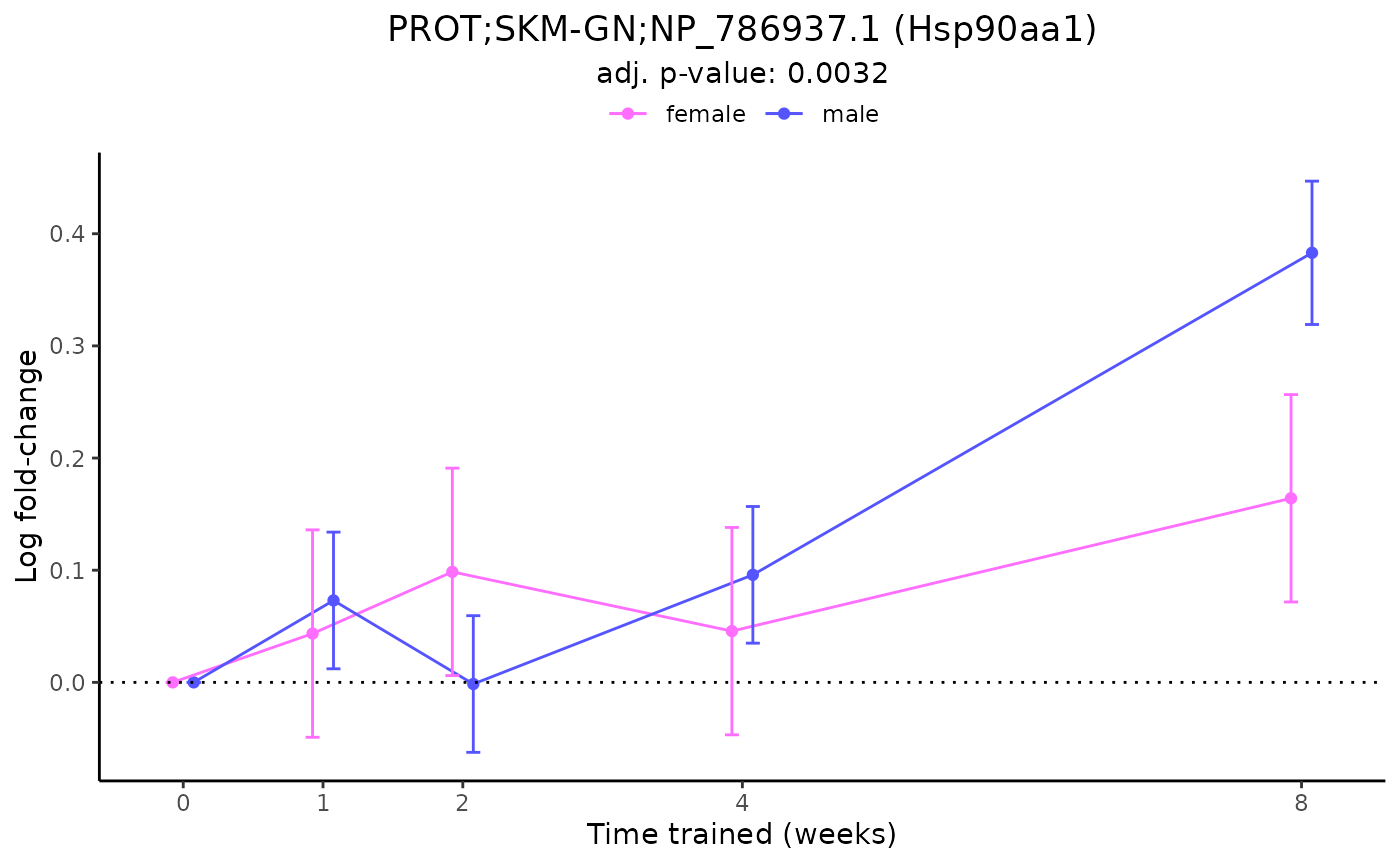


plot_feature_logfc(assay = "PROT",
                   tissue = "SKM-GN",
                   feature_ID = "NP_786937.1",
                   scale_x_by_time = FALSE)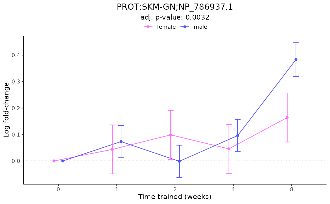


plot_feature_logfc(assay = "PROT",
                   tissue = "SKM-GN",
                   feature_ID = "NP_786937.1",
                   facet_by_sex = TRUE,
                   add_adj_p = FALSE)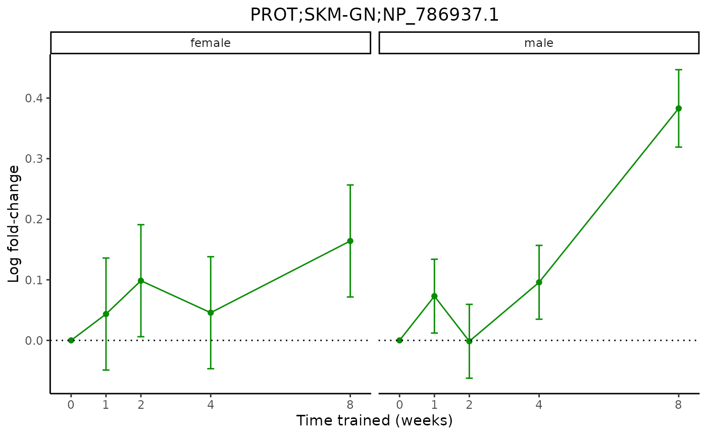

Bayesian graphical clustering

Summary

After performing differential analysis between trained animals and sedentary control animals to identify training-regulated features across datasets, we wanted to characterize groups of these features that had similar trajectories over the training time course and compare them within and between tissues.

To do this, we clustered the 34,244 training-regulated features with complete timewise summary statistics (that is, from all four training time points in both sexes) using their timewise z-scores with the expectation-maximization (EM) clustering algorithm of repfdr. This algorithm assumes that each timewise z-score can take one of three latent states: -1 for down-regulation, 1 for up-regulation, and 0 for null (i.e., unchanged relative to the sedentary control group). The algorithm computes the posterior probabilities for each combination of states (-1/down, 1/up, or 0/null) over all experimental groups (8 groups: 1-, 2-, 4-, and 8-week time points in females and males). We used these posterior probabilities to effectively assign continuous z-scores to simplified states. For example, a feature with the following z-scores would be assigned to the corresponding states with high probability:

	Female 1w	Male 1w	Female 2w	Male 2w	Female 4w	Male 4w	Female 8w	Male 8w
z-score	-0.2	0.1	0.85	-0.05	0.09	6.7	0.21	5
state	0	0	0	0	0	1	0	1

We then combine the male and female states for a given time point using the following notation:

	1 week	2 weeks	4 weeks	8 weeks
notation	`1w_F0_M0`	`2w_F0_M0`	`4w_F0_M1`	`8w_F0_M1`

Descriptively, this feature is null in both sexes (F0_M0) at 1 week (1w) and 2 weeks (2w) of training and up-regulated in males only (F0_M1) at 4 and 8 weeks of training.

One major advantage of this approach is that we can use the time points and discrete states to construct a graph, where each point (or “node”) in the graph represents a state at a given time point (e.g., 1w_F-1_M0). Then for each feature of interest, we can draw a path through the graph to represent its trajectory over the training time course. We can use the paths and nodes in the graph to define clusters of features with similar temporal behavior and characterize the underlying biology.

For example, we can represent the complete path of the above feature over the training time course as follows: 1w_F0_M0->2w_F0_M0->4w_F0_M1->8w_F0_M1. This path is made by connecting the 1w_F0_M0 node to the 2w_F0_M0 node to the 4w_F0_M1 node to the 8w_F0_M1 node. The connection between a single pair of consecutive nodes is called an edge. For example, the 2w_F0_M0---4w_F0_M1 edge represents features that are null in both sexes after 2 weeks of training but are up-regulated in males after 4 weeks of training. The 1w_F0_M0->2w_F0_M0->4w_F0_M1->8w_F0_M1 path is constructed from 3 edges, each represented by -> in the notation.

The figure below provides toy examples of four features to demonstrate their graphical representation. Feature f2 (green) is the same trajectory described above.

A. A schematic example of the graphical representation of the differential analysis results. Top left: the z-scores of four features. A positive score corresponds to up-regulation (red), and a negative score corresponds to down regulation (blue). Bottom left: the assignment of features to node sets and full path sets (edge sets are not shown for conciseness but can be easily inferred from the full paths). Node labels follow the [time]_F[x]_M[y] format where [time] shows the animal sacrifice week and can take one of (1w, 2w, 4w, or 8w), and [x] and [y] are one of (-1,0,1), corresponding to down-regulation, no effect, and up-regulation, respectively. Right: the graphical representation of the feature sets. Columns are training time points, and rows are the differential abundance states. Node and edge sizes are proportional to the number of features that are assigned to each set.

We herein refer to our approach of using repfdr to construct a graph of the dynamic multi-omic responses to endurance exercise training across tissues as graphical clustering. The following sections describe how to reproduce our graphical clustering analysis, run repfdr on your own data, and explore and visualize the nodes, edges, and paths (collectively referred to as clusters) in the resulting graph. For additional details and advantages of this approach over traditional clustering methods, see the supplementary information of our Nature publication. If you are more interested in exploring the existing pathway enrichment results, skip to Visualization of pathway enrichment results.

(Re-)run `repfdr` to determine states

REPFDR_INPUTS provides the inputs for our analysis with repfdr, which can be replicated with bayesian_graphical_clustering() as shown below. The raw repfdr results are provided in REPFDR_RES.

data(REPFDR_INPUTS)
zscores = REPFDR_INPUTS$zs_smoothed
res = bayesian_graphical_clustering(zscores)

bayesian_graphical_clustering() is a study-specific wrapper for repfdr_wrapper(). repfdr_wrapper() can be used to analyze any set of z-scores. Here we show an example with simulated data.

# load required library for this function
library(repfdr)

# Simulate data with a single null cluster
# Toy experiment with 8 groups 
zcolnames = paste("Exp", 1:8)
zscores = matrix(rnorm(80000),ncol=8,dimnames = list(1:10000,zcolnames))
# Add a cluster with a strong signal,
# i.e. assign a z-score of ~5 to the first 4 groups for the first 500 features
zscores[1:500,1:4] = zscores[1:500,1:4] + 5
# Run the repfdr wrapper
repfdr_results = repfdr_wrapper(zscores, df=10)
#> EM iteration 2
#> EM iteration 3
#> EM iteration 4
#> EM iteration 5
#> EM iteration 6
#> EM iteration 7
#> EM iteration 8
#> EM iteration 9
#> EM iteration 10
#> EM iteration 11
#> EM iteration 12
#> EM iteration 13
#> EM iteration 14
#> EM iteration 15
#> EM iteration 16
#> EM iteration 17
#> EM iteration 18
#> EM iteration 19
#> EM iteration 20
#> EM iteration 21
#> EM iteration 22
#> EM iteration 23
#> EM iteration 24
#> EM iteration 25
#> EM iteration 26
#> EM iteration 27
#> EM iteration 28
#> EM iteration 29
#> EM iteration 30
#> EM iteration 31
#> EM iteration 32
#> EM iteration 33
#> EM iteration 34
#> EM iteration 35
#> EM iteration 36
#> EM iteration 37
#> EM iteration 38
#> EM iteration 39
#> EM iteration 40
#> EM iteration 41
#> EM iteration 42
#> EM iteration 43
#> EM iteration 44
#> EM iteration 45
#> EM iteration 46
#> EM iteration 47
#> EM iteration 48
#> EM iteration 49
#> EM iteration 50
#> EM iteration 51
#> EM iteration 52
#> EM iteration 53
#> EM iteration 54
#> EM iteration 55
#> EM iteration 56
#> EM iteration 57
#> EM iteration 58
#> EM iteration 59
#> EM iteration 60
#> EM iteration 61
#> EM iteration 62
#> EM iteration 63
#> EM iteration 64
#> EM iteration 65
#> EM iteration 66
#> EM iteration 67
#> EM iteration 68
#> EM iteration 69
#> EM iteration 70
#> EM iteration 71
#> EM iteration 72
#> EM iteration 73
#> EM iteration 74
#> EM iteration 75
#> EM iteration 76
#> EM iteration 77
#> EM iteration 78
#> EM iteration 79
#> EM iteration 80
#> EM iteration 81
#> EM iteration 82
#> EM iteration 83
#> EM iteration 84
#> EM iteration 85
#> EM iteration 86
#> EM iteration 87
#> EM iteration 88
#> EM iteration 89
#> EM iteration 90
#> EM iteration 91
#> EM iteration 92
#> EM iteration 93
#> EM iteration 94
#> EM iteration 95
#> EM iteration 96
#> EM iteration 97
#> EM iteration 98
#> EM iteration 99
#> EM iteration 100
#> EM iteration 101
#> EM iteration 102
#> EM iteration 103
#> EM iteration 104
#> EM iteration 105
#> EM iteration 106
#> EM iteration 107
#> EM iteration 108
#> EM iteration 109
#> EM iteration 110
#> EM iteration 111
#> EM iteration 112
#> EM iteration 113
#> EM iteration 114
#> EM iteration 115
#> EM iteration 116
#> EM iteration 117
#> EM iteration 118
#> EM iteration 119
#> EM iteration 120
#> EM iteration 121
#> EM iteration 122
#> EM iteration 123
#> EM iteration 124
#> EM iteration 125
#> EM iteration 126
#> EM iteration 127
#> EM iteration 128
#> EM iteration 129
#> EM iteration 130
#> EM iteration 131
#> EM iteration 132
#> EM iteration 133
#> EM iteration 134
#> EM iteration 135
#> EM iteration 136
#> EM iteration 137
#> EM iteration 138
#> EM iteration 139
#> EM iteration 140
#> EM iteration 141
#> EM iteration 142
#> EM iteration 143
#> EM iteration 144
#> EM iteration 145
#> EM iteration 146
#> EM iteration 147
#> EM iteration 148
#> EM iteration 149
#> EM iteration 150
#> EM iteration 151
#> EM iteration 152
#> EM iteration 153
#> EM iteration 154
#> EM iteration 155
#> EM iteration 156
#> EM iteration 157
#> EM iteration 158
#> EM iteration 159
#> EM iteration 160
#> EM iteration 161
#> EM iteration 162
#> EM iteration 163
#> EM iteration 164
#> EM iteration 165
#> EM iteration 166
#> EM iteration 167
#> EM iteration 168
#> EM iteration 169
#> EM iteration 170
#> EM iteration 171
#> EM iteration 172
#> EM iteration 173
#> EM iteration 174
#> EM iteration 175
#> EM iteration 176
#> EM iteration 177
#> EM iteration 178
#> EM iteration 179
#> EM iteration 180
#> EM iteration 181
#> EM iteration 182
#> EM iteration 183
#> EM iteration 184
#> EM iteration 185
#> EM iteration 186
#> EM iteration 187
#> EM iteration 188
#> EM iteration 189
#> EM iteration 190
#> EM iteration 191
#> EM iteration 192
#> EM iteration 193
#> EM iteration 194
#> EM iteration 195
#> EM iteration 196
#> EM iteration 197
#> EM iteration 198
#> EM iteration 199
#> EM iteration 200
#> EM iteration 201
#> EM iteration 202
#> EM iteration 203
#> EM iteration 204
#> EM iteration 205
#> EM iteration 206
#> EM iteration 207
#> EM iteration 208
#> EM iteration 209
#> EM iteration 210
#> EM iteration 211
#> EM iteration 212
#> EM iteration 213
#> EM iteration 214
#> EM iteration 215
#> EM iteration 216
#> EM iteration 217
#> EM iteration 218
#> EM iteration 219
#> EM iteration 220
#> EM iteration 221
#> EM iteration 222
#> EM iteration 223
#> EM iteration 224
#> EM iteration 225
#> EM iteration 226
#> EM iteration 227
#> EM iteration 228
#> EM iteration 229
#> EM iteration 230
#> EM iteration 231
#> EM iteration 232
#> EM iteration 233
#> EM iteration 234
#> EM iteration 235
#> EM iteration 236
#> EM iteration 237
#> EM iteration 238
#> EM iteration 239
#> EM iteration 240
#> EM iteration 241
#> EM iteration 242
#> EM iteration 243
#> EM iteration 244
#> EM iteration 245
#> EM iteration 246
#> EM iteration 247
#> EM iteration 248
#> EM iteration 249
#> EM iteration 250
#> EM iteration 251
#> EM iteration 252
#> EM iteration 253
#> EM iteration 254
#> EM iteration 255
#> EM iteration 256
#> EM iteration 257
#> EM iteration 258
#> EM iteration 259
#> EM iteration 260
#> EM iteration 261
#> EM iteration 262
#> EM iteration 263
#> EM iteration 264
#> EM iteration 265
#> EM iteration 266
#> EM iteration 267
#> EM iteration 268
#> EM iteration 269
#> EM iteration 270
#> EM iteration 271
#> EM iteration 272
#> EM iteration 273
#> EM iteration 274
#> EM iteration 275
#> EM iteration 276
#> EM iteration 277
#> EM iteration 278
#> EM iteration 279
#> EM iteration 280
#> EM iteration 281
#> EM iteration 282
#> EM iteration 283
#> EM iteration 284
#> EM iteration 285
#> EM iteration 286
#> EM iteration 287
#> EM iteration 288
#> EM iteration 289
#> EM iteration 290
#> EM iteration 291
#> EM iteration 292
#> EM iteration 293
#> EM iteration 294
#> Converged after 293 EM iterations.

# Now we expect the first 500 features to belong to cluster 11110000 (up-regulated in the first 4 groups)
# and the remaining 9500 to belong to cluster 00000000 (null in all groups)
hist(repfdr_results$repfdr_cluster_posteriors[,"00000000"], 
     breaks=20, 
     main="Posterior probability of null cluster for all features")

hist(repfdr_results$repfdr_cluster_posteriors[1:500,"11110000"], 
     breaks=20, 
     main="Posterior probability of 11110000 cluster for first 500 features")

Explore graphical clustering results

The graph representation of the repfdr results are provided in GRAPH_COMPONENTS (node and edge lists) and GRAPH_STATES (data frame representation).

data(GRAPH_STATES)
head(GRAPH_STATES)
#>                                                             feature    ome
#> ACETYL;HEART;NP_001003673.1_K477k ACETYL;HEART;NP_001003673.1_K477k ACETYL
#> ACETYL;HEART;NP_001004072.2_K77k   ACETYL;HEART;NP_001004072.2_K77k ACETYL
#> ACETYL;HEART;NP_001004072.2_K83k   ACETYL;HEART;NP_001004072.2_K83k ACETYL
#> ACETYL;HEART;NP_001004085.1_K186k ACETYL;HEART;NP_001004085.1_K186k ACETYL
#> ACETYL;HEART;NP_001004085.1_K261k ACETYL;HEART;NP_001004085.1_K261k ACETYL
#> ACETYL;HEART;NP_001004085.1_K268k ACETYL;HEART;NP_001004085.1_K268k ACETYL
#>                                   tissue           feature_ID state_1w state_2w
#> ACETYL;HEART;NP_001003673.1_K477k  HEART NP_001003673.1_K477k    F0_M0    F0_M0
#> ACETYL;HEART;NP_001004072.2_K77k   HEART  NP_001004072.2_K77k    F0_M0    F0_M0
#> ACETYL;HEART;NP_001004072.2_K83k   HEART  NP_001004072.2_K83k  F-1_M-1  F-1_M-1
#> ACETYL;HEART;NP_001004085.1_K186k  HEART NP_001004085.1_K186k    F0_M1    F0_M1
#> ACETYL;HEART;NP_001004085.1_K261k  HEART NP_001004085.1_K261k    F0_M1    F0_M1
#> ACETYL;HEART;NP_001004085.1_K268k  HEART NP_001004085.1_K268k    F0_M1    F0_M1
#>                                   state_4w state_8w
#> ACETYL;HEART;NP_001003673.1_K477k    F0_M0  F-1_M-1
#> ACETYL;HEART;NP_001004072.2_K77k     F1_M0    F1_M0
#> ACETYL;HEART;NP_001004072.2_K83k    F0_M-1    F0_M0
#> ACETYL;HEART;NP_001004085.1_K186k    F0_M0   F0_M-1
#> ACETYL;HEART;NP_001004085.1_K261k    F0_M0   F0_M-1
#> ACETYL;HEART;NP_001004085.1_K268k    F0_M0   F0_M-1
#>                                                                          path
#> ACETYL;HEART;NP_001003673.1_K477k    1w_F0_M0->2w_F0_M0->4w_F0_M0->8w_F-1_M-1
#> ACETYL;HEART;NP_001004072.2_K77k       1w_F0_M0->2w_F0_M0->4w_F1_M0->8w_F1_M0
#> ACETYL;HEART;NP_001004072.2_K83k  1w_F-1_M-1->2w_F-1_M-1->4w_F0_M-1->8w_F0_M0
#> ACETYL;HEART;NP_001004085.1_K186k     1w_F0_M1->2w_F0_M1->4w_F0_M0->8w_F0_M-1
#> ACETYL;HEART;NP_001004085.1_K261k     1w_F0_M1->2w_F0_M1->4w_F0_M0->8w_F0_M-1
#> ACETYL;HEART;NP_001004085.1_K268k     1w_F0_M1->2w_F0_M1->4w_F0_M0->8w_F0_M-1
#>                                                                         tissue_path
#> ACETYL;HEART;NP_001003673.1_K477k    HEART:1w_F0_M0->2w_F0_M0->4w_F0_M0->8w_F-1_M-1
#> ACETYL;HEART;NP_001004072.2_K77k       HEART:1w_F0_M0->2w_F0_M0->4w_F1_M0->8w_F1_M0
#> ACETYL;HEART;NP_001004072.2_K83k  HEART:1w_F-1_M-1->2w_F-1_M-1->4w_F0_M-1->8w_F0_M0
#> ACETYL;HEART;NP_001004085.1_K186k     HEART:1w_F0_M1->2w_F0_M1->4w_F0_M0->8w_F0_M-1
#> ACETYL;HEART;NP_001004085.1_K261k     HEART:1w_F0_M1->2w_F0_M1->4w_F0_M0->8w_F0_M-1
#> ACETYL;HEART;NP_001004085.1_K268k     HEART:1w_F0_M1->2w_F0_M1->4w_F0_M0->8w_F0_M-1

Note: Features are specified in the format “[ASSAY_ABBREV];[TISSUE_ABBREV];[feature_ID]”, e.g. “PHOSPHO;SKM-GN;NP_001006973.1_S34s”, “METAB;SKM-GN;1-methylnicotinamide”

We can extract node, edge, and path feature sets from a given tissue using extract_tissue_sets(). Here we extract training-regulated features in the three (k=3) largest nodes, edges, and paths in the gastrocnemius (tissues="SKM-GN") that have at least 20 features (min_size=20). We also add the feature lists for all 8-week nodes (add_week8=TRUE), which are generally of interest because the 8-week time point represents the final trained state.

gastroc_sets = extract_tissue_sets(tissues="SKM-GN",
                                   k=3,
                                   min_size=20,
                                   add_week8=TRUE)
names(gastroc_sets)
#>  [1] "8w_F1_M1"                                      
#>  [2] "8w_F-1_M-1"                                    
#>  [3] "4w_F1_M1"                                      
#>  [4] "8w_F-1_M0"                                     
#>  [5] "8w_F0_M-1"                                     
#>  [6] "8w_F0_M0"                                      
#>  [7] "8w_F0_M1"                                      
#>  [8] "8w_F1_M0"                                      
#>  [9] "4w_F1_M1---8w_F1_M1"                           
#> [10] "1w_F0_M0---2w_F0_M0"                           
#> [11] "4w_F-1_M-1---8w_F-1_M-1"                       
#> [12] "1w_F1_M1->2w_F1_M1->4w_F1_M1->8w_F1_M1"        
#> [13] "1w_F-1_M-1->2w_F-1_M-1->4w_F-1_M-1->8w_F-1_M-1"
#> [14] "1w_F0_M1->2w_F0_M1->4w_F1_M1->8w_F1_M1"

# look at the list of features in the "1w_F1_M1->2w_F1_M1->4w_F1_M1->8w_F1_M1" path
head(gastroc_sets$`1w_F1_M1->2w_F1_M1->4w_F1_M1->8w_F1_M1`)
#> [1] "ATAC;SKM-GN;chr15:101579022-101579761"
#> [2] "ATAC;SKM-GN;chr1:221194280-221195125" 
#> [3] "ATAC;SKM-GN;chr1:221199295-221200124" 
#> [4] "ATAC;SKM-GN;chr20:34579127-34579734"  
#> [5] "ATAC;SKM-GN;chr5:114013062-114014681" 
#> [6] "ATAC;SKM-GN;chrX:119151643-119154560"

get_all_trajectories() returns all non-empty paths in the results.

paths = get_all_trajectories()
head(names(paths))
#> [1] "1w_F-1_M1->2w_F-1_M0->4w_F-1_M0->8w_F-1_M0"
#> [2] "1w_F0_M1->2w_F0_M1->4w_F0_M1->8w_F1_M1"    
#> [3] "1w_F1_M1->2w_F1_M1->4w_F1_M1->8w_F1_M1"    
#> [4] "1w_F0_M0->2w_F0_M0->4w_F0_M0->8w_F1_M1"    
#> [5] "1w_F0_M0->2w_F0_M0->4w_F0_M0->8w_F-1_M-1"  
#> [6] "1w_F0_M1->2w_F0_M1->4w_F0_M1->8w_F0_M1"
hist(unlist(lapply(paths, length)), breaks=100)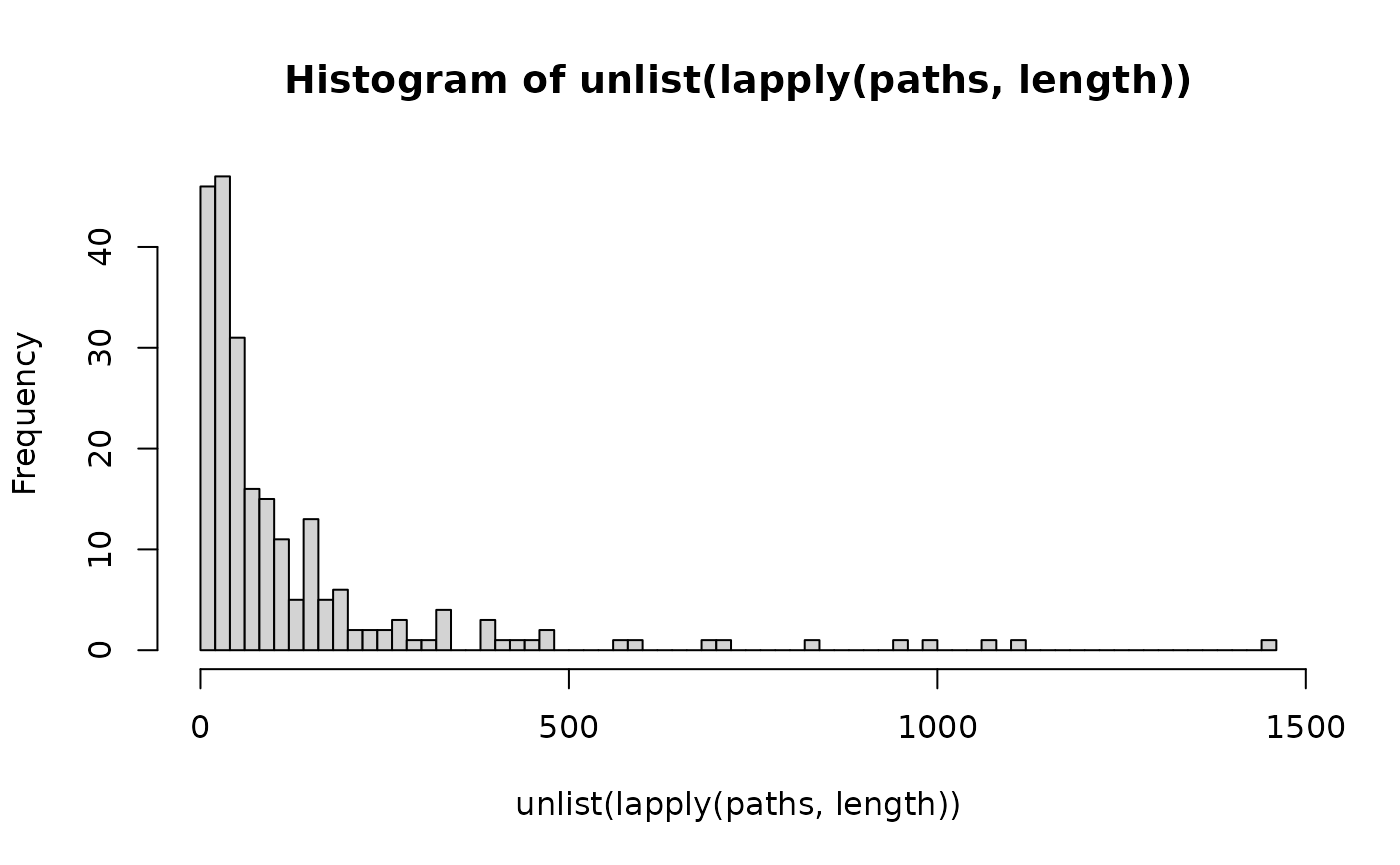

extract_main_clusters() returns the subset of graphical clusters for which pathway enrichment was performed for the Nature publication, namely the 2 largest nodes, 2 largest edges, 10 largest non-null paths, and all 8-week nodes from the graphical representation of training-regulated features in each tissue.

clusters = extract_main_clusters()

To extract the training-regulated features associated with a specific graphical cluster, tissue, ome, etc., we can subset GRAPH_STATES.

data(GRAPH_STATES)

# if you want features in this path in LUNG:
clust = "LUNG:1w_F1_M-1->2w_F1_M-1->4w_F0_M-1->8w_F-1_M-1"
features_of_interest = stats::na.omit(GRAPH_STATES$feature[GRAPH_STATES$tissue_path == clust])
as.vector(features_of_interest)
#>  [1] "PHOSPHO;LUNG;NP_001012023.1_S447s"     
#>  [2] "PHOSPHO;LUNG;NP_001013238.2_S1594s"    
#>  [3] "PHOSPHO;LUNG;NP_001020859.1_S486sS489s"
#>  [4] "PHOSPHO;LUNG;NP_001028859.1_S133s"     
#>  [5] "PHOSPHO;LUNG;NP_001099225.2_S621s"     
#>  [6] "PHOSPHO;LUNG;NP_001099344.2_S1816s"    
#>  [7] "PHOSPHO;LUNG;NP_001164067.1_T456t"     
#>  [8] "PHOSPHO;LUNG;NP_001178760.1_S542s"     
#>  [9] "PHOSPHO;LUNG;NP_001178775.1_S270s"     
#> [10] "PHOSPHO;LUNG;NP_001178880.1_S5423s"    
#> [11] "PHOSPHO;LUNG;NP_036849.1_T422t"        
#> [12] "PHOSPHO;LUNG;NP_037349.1_S512s"        
#> [13] "PHOSPHO;LUNG;NP_058862.1_S63s"         
#> [14] "PHOSPHO;LUNG;NP_647546.1_S288s"        
#> [15] "PHOSPHO;LUNG;NP_665709.2_S702s"        
#> [16] "PHOSPHO;LUNG;XP_001058477.1_S2558s"    
#> [17] "PHOSPHO;LUNG;XP_002726994.2_S307s"     
#> [18] "PHOSPHO;LUNG;XP_003752547.1_S411s"     
#> [19] "PHOSPHO;LUNG;XP_003752548.1_S411s"     
#> [20] "PHOSPHO;LUNG;XP_003754609.1_S1206s"    
#> [21] "PHOSPHO;LUNG;XP_006226323.1_Y618y"     
#> [22] "PHOSPHO;LUNG;XP_006235089.1_S434s"     
#> [23] "PHOSPHO;LUNG;XP_008766933.1_S1807s"    
#> [24] "PHOSPHO;LUNG;XP_017443701.1_S938s"     
#> [25] "PHOSPHO;LUNG;XP_017444244.1_S5362s"    
#> [26] "PHOSPHO;LUNG;XP_017454714.1_S1250s"    
#> [27] "PHOSPHO;LUNG;XP_017454716.1_S1225s"    
#> [28] "PHOSPHO;LUNG;XP_017457486.1_S406s"     
#> [29] "PHOSPHO;LUNG;XP_017457774.1_S758s"     
#> [30] "PROT;LUNG;XP_003750594.1"

# if you want features in this path in multiple tissues:
clust = "1w_F1_M1->2w_F1_M1->4w_F1_M1->8w_F1_M1"
tissues = c("HEART","SKM-GN","SKM-VL")
features_of_interest = stats::na.omit(GRAPH_STATES$feature[GRAPH_STATES$path == clust & GRAPH_STATES$tissue %in% tissues])
length(features_of_interest)
#> [1] 685
# look at a table of omes and tissues represented 
tissues = sapply(features_of_interest, function(x){
  unname(unlist(strsplit(x, ";")))[2]
})
omes = sapply(features_of_interest, function(x){
  unname(unlist(strsplit(x, ";")))[1]
})
table(tissues, omes)
#>         omes
#> tissues  ACETYL ATAC METAB PHOSPHO PROT TRNSCRPT UBIQ
#>   HEART      50    0    35      52  108      110    2
#>   SKM-GN      0    6    14      55  130       44    0
#>   SKM-VL      0    0     2       0    0       77    0

Plot graph of differential features

We can use get_tree_plot_for_tissue() to draw the graphical representation of a given set of training-regulated features.

First, let’s look at the graph of all differential features in the liver. The sizes of the edges and nodes are proportional to the number of training-regulated features that were assigned to the corresponding states. Nodes are arranged in rows by states (e.g., “F only up”) and in columns by training time points. The node at the intersection of “F only up” and “week 1” represents features that are null in males and up-regulated in females after one week of endurance exercise training (i.e., 1w_F1_M0 in the notation above).

get_tree_plot_for_tissue(
  tissues=c("LIVER"),
  min_size = 1
)
#> Using "sugiyama" as default layout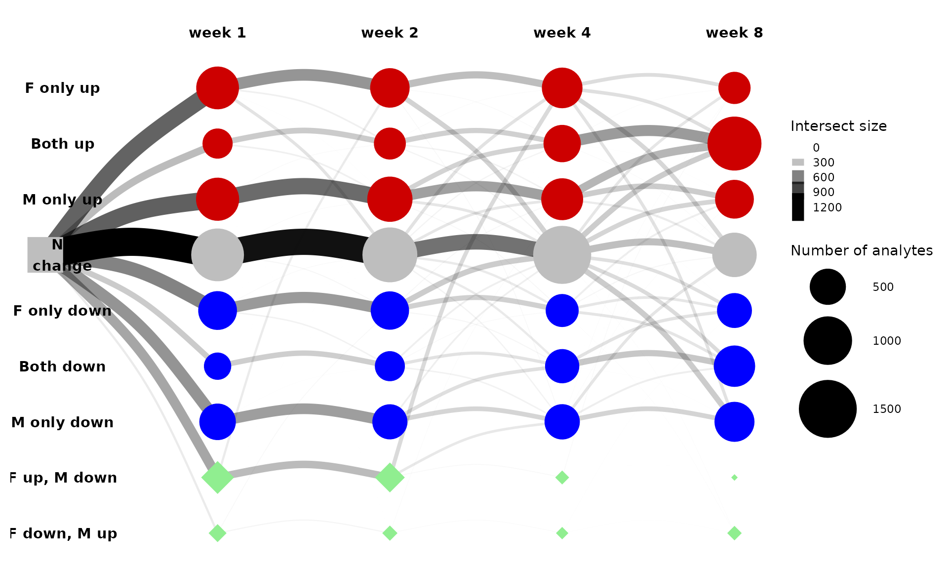

This is messy, so let’s look at just the 5 largest paths instead.

get_tree_plot_for_tissue(
  tissues=c("LIVER"),
  max_trajectories = 5
)
#> Using "sugiyama" as default layout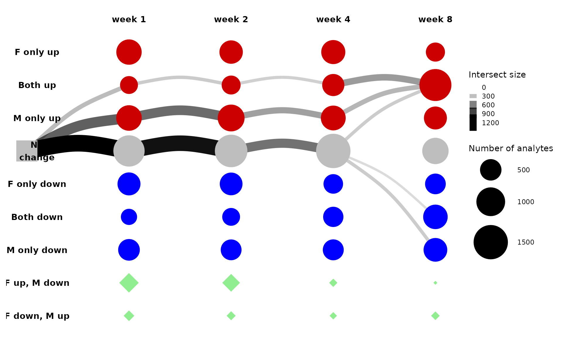

Further, let’s split these edges by data type (assay/ome) to see what features are represented. We can change the curvature and alpha range to make the edges easier to see.

get_tree_plot_for_tissue(
  tissues=c("LIVER"),
  max_trajectories = 5,
  parallel_edges_by_ome = TRUE,
  curvature = 0.5,
  edge_alpha_range = c(0.5,1)
)
#> Using "sugiyama" as default layout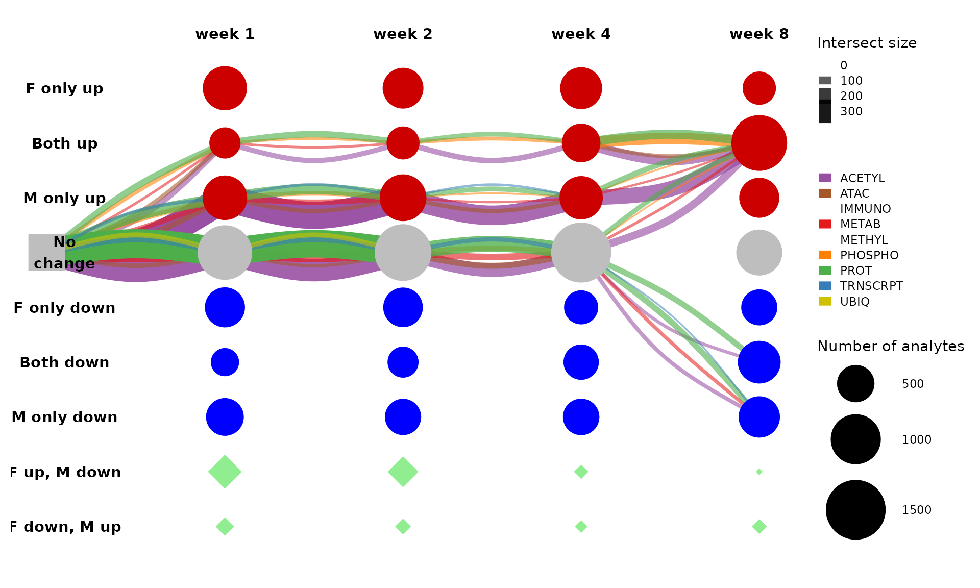

This is too busy with edges split by ome. Let’s look at just the largest path and only RNA-Seq and proteomics assays.

get_tree_plot_for_tissue(
  omes=c("PROT","ACETYL","UBIQ","PHOSPHO","TRNSCRPT"),
  tissues=c("LIVER"),
  max_trajectories = 1,
  parallel_edges_by_ome = TRUE,
  curvature = 0.8,
  edge_alpha_range = c(0.5,1)
)
#> Using "sugiyama" as default layout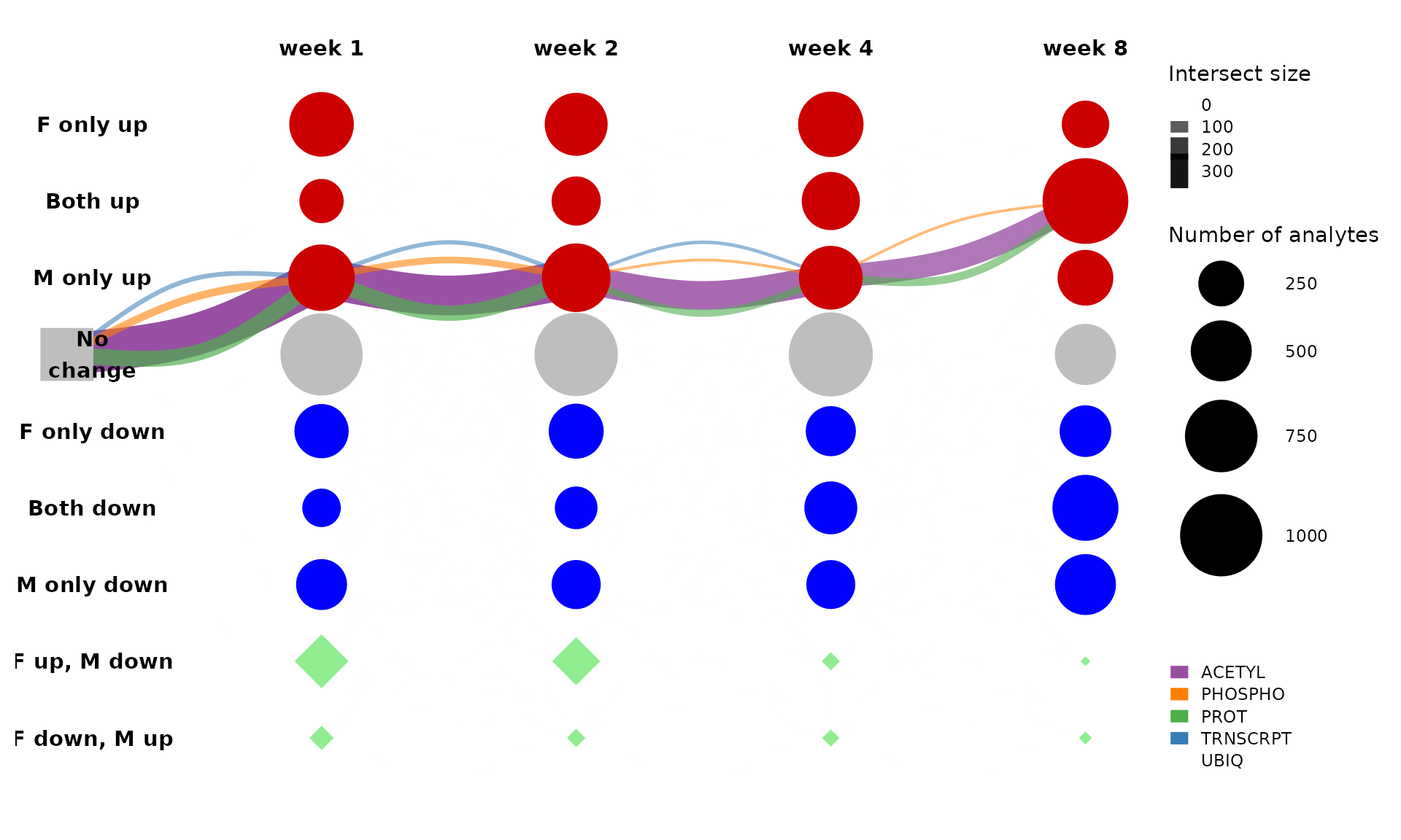

From this plot, we can see that most of the differential features that follow this path in the liver are protein acetlysites. This path represents features that are up-regulated only in males (“M only up”) through the first four weeks of training and then in both males and females by eight weeks of training (“Both up”).

We can also look at multi-tissue graphs. For example, let’s look at the three largest paths of training-regulated transcripts in the three muscle tissues. Now instead of splitting edges by ome, we can split them by tissue.

get_tree_plot_for_tissue(
  tissues=c("SKM-GN","HEART","SKM-VL"),
  omes="TRNSCRPT",
  parallel_edges_by_tissue = TRUE,
  max_trajectories = 3,
  edge_alpha_range = c(0.5,1),
  curvature = 0.6
)
#> Using "sugiyama" as default layout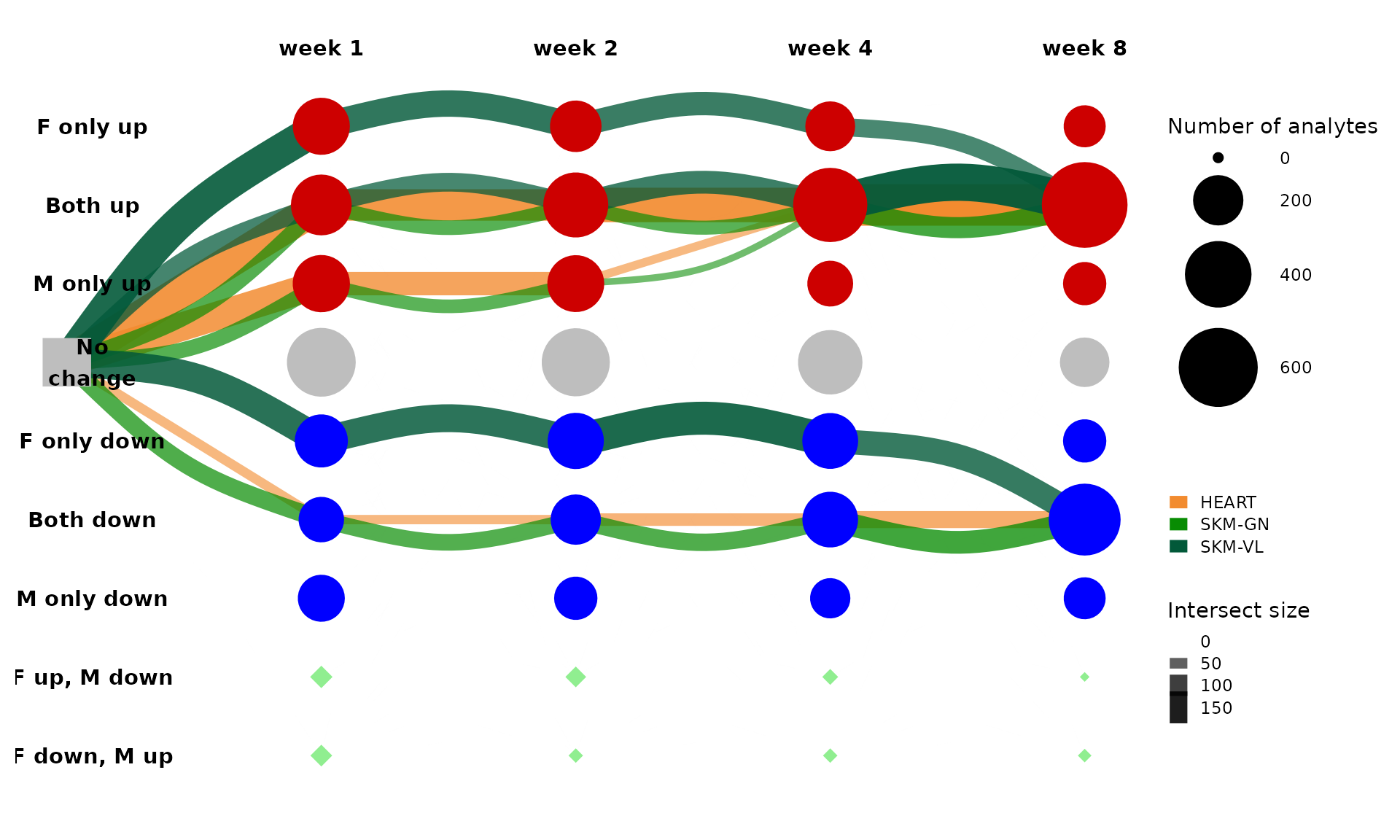

From this plot, we can see that a large number of training-regulated transcripts are up-regulated in both sexes at all four training time points in all three muscle tissues. Perhaps some interesting shared biology is represented in muscle features that follow this path.

To visualize the representation of features from different tissues and/or omes for a given set of clusters, we can also use plot_features_per_cluster(). Here, we’ll consider the 10 largest paths of training-regulated features in the gastrocnemius (lower leg skeletal muscle).

# Get top 10 largest paths, nodes, edges in gastrocnemius
# Exclude additional 8-week nodes
clusters = extract_tissue_sets("SKM-GN", k=10, add_week8=FALSE)
# Select paths only
clusters = clusters[grepl("->", names(clusters))]
# Plot distribution of features
plot_features_per_cluster(clusters)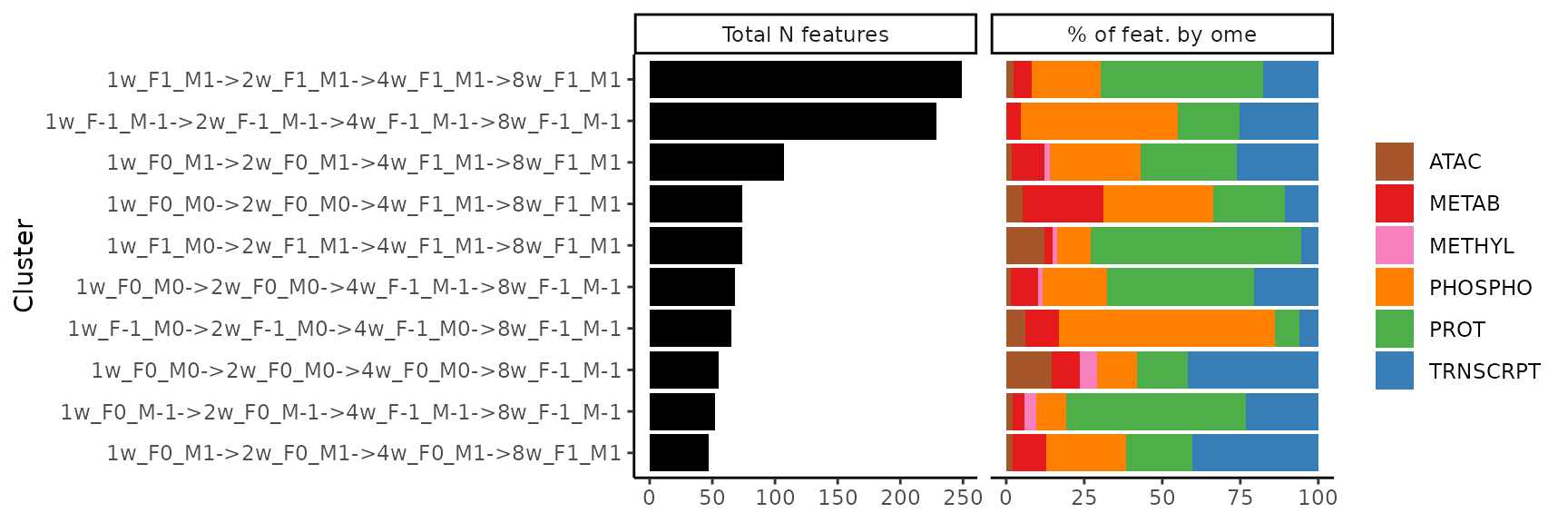

From this plot, we see that the majority of training-regulated features in the gastrocnemius that are up-regulated in both sexes at all training time points (1w_F1_M1->2w_F1_M1->4w_F1_M1->8w_F1_M1, top row) are proteins, followed by protein phosphosites. We can plot the sample-level trajectories of all features in this cluster with plot_feature_trajectories().

plot_feature_trajectories(clusters$`1w_F1_M1->2w_F1_M1->4w_F1_M1->8w_F1_M1`, 
                          title="Features consistently up-regulated in gastroc")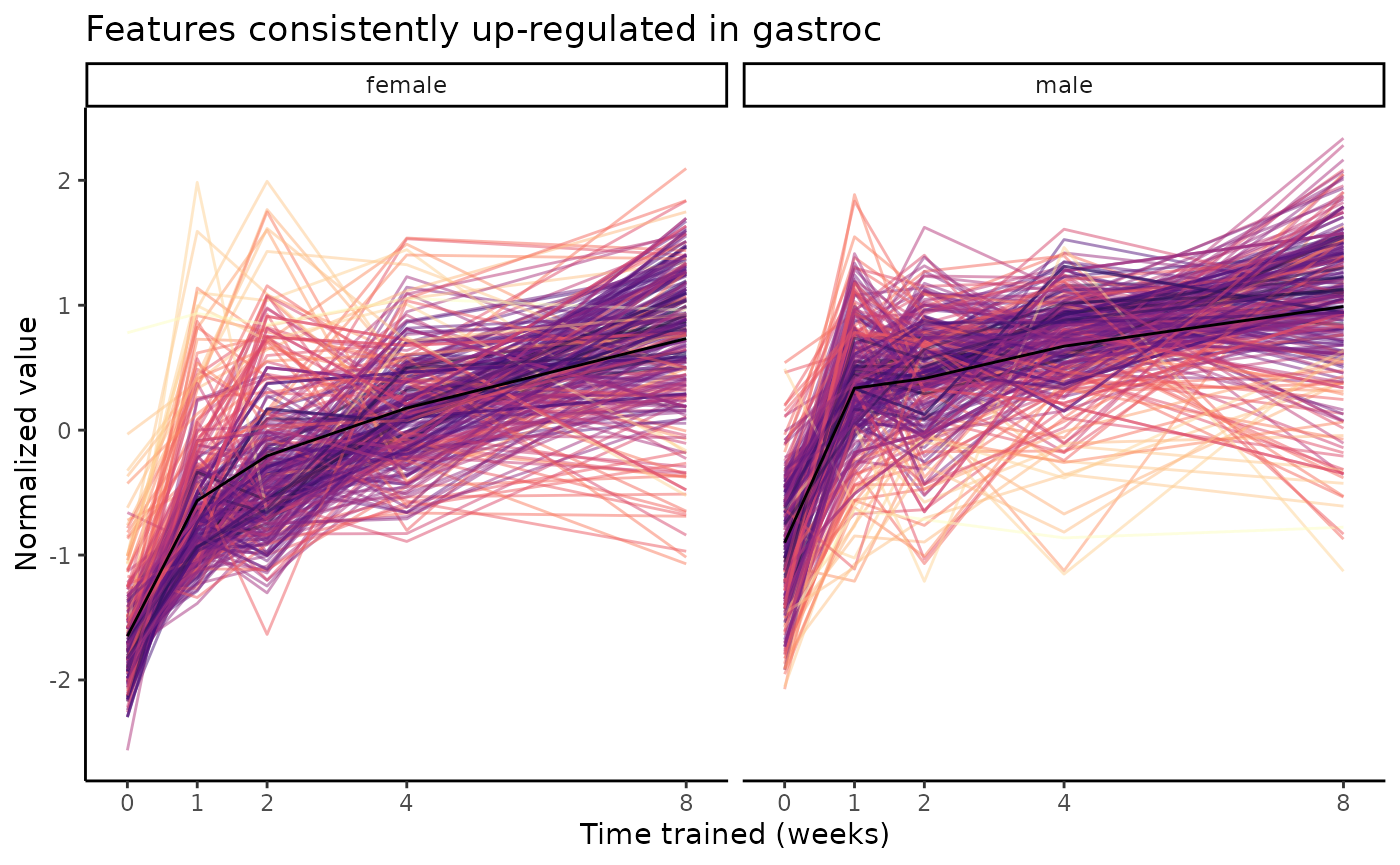

We also see a cluster comprised mostly of protein phosphosites, where these features are down-regulated in females at all training time points and also down-regulated in males at 8 weeks of training (1w_F-1_M0->2w_F-1_M0->4w_F-1_M0->8w_F-1_M-1).

plot_feature_trajectories(clusters$`1w_F-1_M0->2w_F-1_M0->4w_F-1_M0->8w_F-1_M-1`, 
                          title="Cluster of mostly PHOSPHO in gastroc")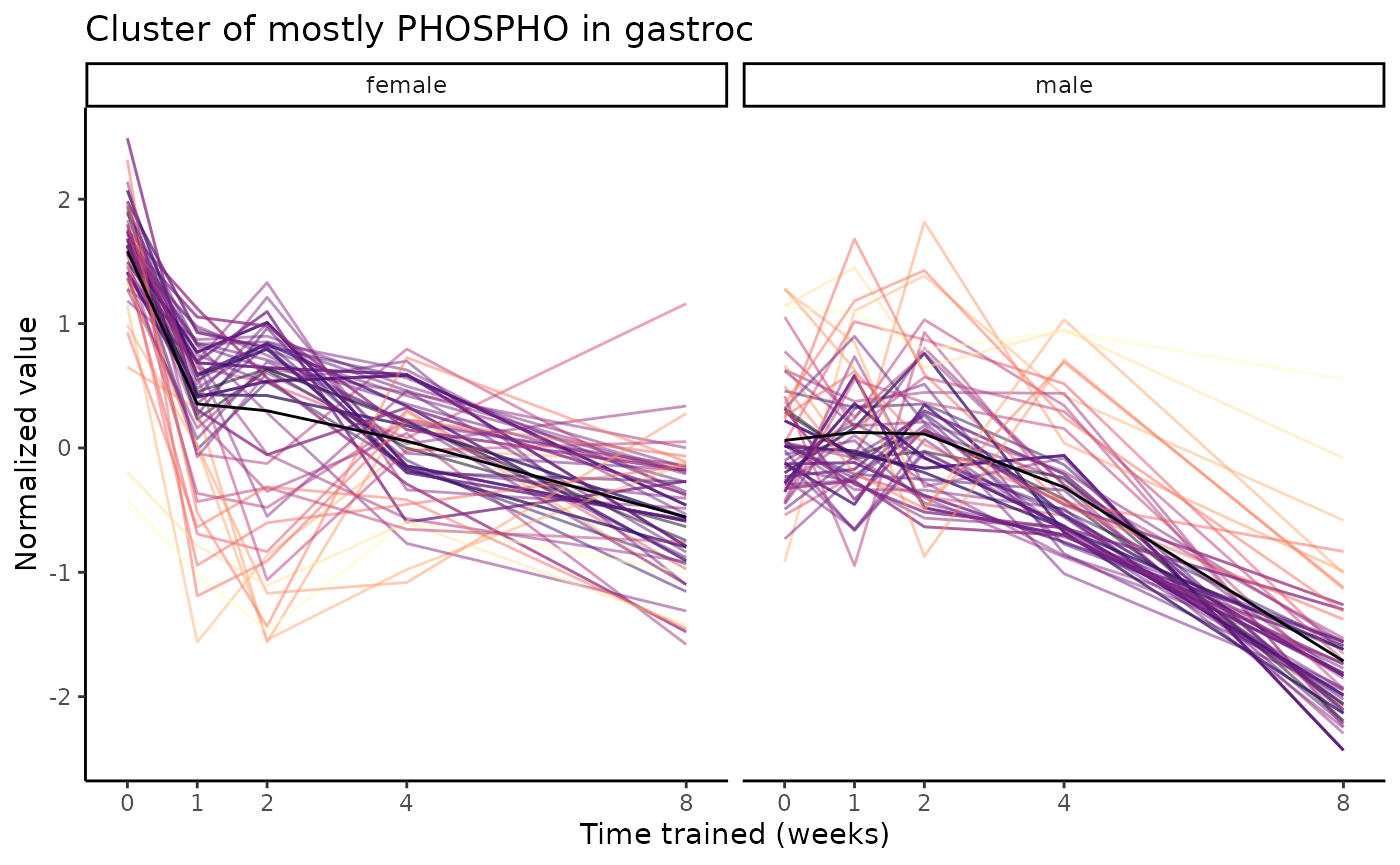

In the next section, we show how pathway enrichment can be used to begin interpreting the biology underlying a graphical cluster (node, edge, or path) of interest.

Pathway enrichment of clusters

One important tool we used to interpret the biology underlying graphical clusters was pathway enrichment. In this section, we describe functions provided in this package to reproduce our pathway enrichment analysis or run your own. If you are more interested in exploring the existing pathway enrichment results, skip to Visualization of pathway enrichment results.

Approach

We performed pathway enrichment for the 2 largest nodes, 2 largest edges, 10 largest non-null paths, and all 8-week nodes from the graphical representation of training-regulated features in each tissue. This set of graphical clusters can be extracted using extract_main_clusters().

For each tissue-specific cluster, we performed pathway enrichment separately for the features corresponding to each ome. For gene-centric omes, i.e., all but metabolomics, we mapped features to genes and queried KEGG and REACTOME pathways using gprofiler2. For metabolomics, we mapped metabolites to KEGG IDs and used FELLA to query KEGG pathways. The feature-to-gene and metabolite-to-KEGG ID mappings are provided in FEATURE_TO_GENE.

For each enrichment test, we specified the background/universe as the set of genes or metabolite IDs that were tested for differential analysis in that tissue. These backgrounds are provided in GENE_UNIVERSES. If you are performing your own pathway enrichment analyses, it is important to specify the appropriate background to avoid artificially small p-values.

Pathway enrichment results were adjusted over all tests using IHW with tissue as a covariate.

Pathway enrichment results for graphical clusters of interest presented in our publication are provided in GRAPH_PW_ENRICH.

Enrichment with standard PWs

cluster_pathway_enrichment() is a wrapper for gprofiler2::gost() and FELLA::enrich(), where metabolomics pathway enrichment is performed for KEGG pathways, and gene-centric pathway enrichment can be performed for any set of pathway databases accepted by g:Profiler.

Here we show an example of performing pathway enrichment on two clusters of training-regulated features, one from each of two tissues. In this case, clusters are determined using the graphical clustering approach described above, but in practice the clusters could be identified using any approach (e.g., k-means, fuzzy C-means).

First, extract the clusters of interest. Here paths is a named list, where the names are the names of the cluster and the values are vectors of the corresponding training-regulated features.

# extract the top path from gastrocnemius and heart 
paths = list()
for (tissue in c("SKM-GN","HEART")){
  # extract top node, edge, path
  clusters = extract_tissue_sets(tissue, k=1, add_week8=FALSE)
  # select the path only, which contains "->"
  top_path = clusters[grepl("->", names(clusters))]
  # add to list 
  paths[[paste0(tissue, ":", names(top_path)[1])]] = top_path[[1]]
}
names(paths)
#> [1] "SKM-GN:1w_F1_M1->2w_F1_M1->4w_F1_M1->8w_F1_M1"
#> [2] "HEART:1w_F1_M1->2w_F1_M1->4w_F1_M1->8w_F1_M1"
lapply(paths, head)
#> $`SKM-GN:1w_F1_M1->2w_F1_M1->4w_F1_M1->8w_F1_M1`
#> [1] "ATAC;SKM-GN;chr15:101579022-101579761"
#> [2] "ATAC;SKM-GN;chr1:221194280-221195125" 
#> [3] "ATAC;SKM-GN;chr1:221199295-221200124" 
#> [4] "ATAC;SKM-GN;chr20:34579127-34579734"  
#> [5] "ATAC;SKM-GN;chr5:114013062-114014681" 
#> [6] "ATAC;SKM-GN;chrX:119151643-119154560" 
#> 
#> $`HEART:1w_F1_M1->2w_F1_M1->4w_F1_M1->8w_F1_M1`
#> [1] "ACETYL;HEART;NP_001004220.1_K116k" "ACETYL;HEART;NP_001006973.1_K401k"
#> [3] "ACETYL;HEART;NP_001007621.1_K354k" "ACETYL;HEART;NP_001014183.1_K193k"
#> [5] "ACETYL;HEART;NP_001014183.1_K199k" "ACETYL;HEART;NP_001030123.1_K581k"

Now perform pathway enrichment. First, we will run the function without specifying kegg_db_destination, which will force it to ignore metabolites. By default, KEGG and REACTOME pathways are queried.

# load required libraries for this function
library(gprofiler2)
library(foreach)
# to learn more about the arguments and default parameters, look at `?cluster_pathway_enrichment`
res1 = cluster_pathway_enrichment(paths)
#> Warning in cluster_pathway_enrichment(paths): It looks like you have metabolites in your clustering result, but you did not provide a path for the KEGG database ('kegg_db_destination'). Pathway enrichment will be skipped for metabolites.
#> Number of cores not defined with 'num_cores' argument. Setting the number of cores to 1. Explicity define 'num_cores' to take advantage of parallelization. If you aren't sure how many cores are available to you, try 'length(parallel::mcaffinity()).'
#> Running enrichments for 11 gene sets on 1 core(s). This may take a while...
#> 
#> 1 out of 6 identifiers in SKM-GN:1w_F1_M1->2w_F1_M1->4w_F1_M1->8w_F1_M1 ATAC SKM-GN are not in the current universe. Removing these features.
#> [1] "ENSRNOG00000052048"
#> Done.
#> We recommend that you supply (many) more than 1000 p-values for meaningful data-driven hypothesis weighting results.

We get a few warnings and messages.

First, we get a warning that pathway enrichment will not be performed with metabolites because kegg_db_destination=NULL (default parameter).
Second, we are told that the analysis will be run on a single core. If you are performing pathway enrichment for more than a few clusters, the runtime will be dramatically reduced if you parallelize the analysis on more than one core. You can do this by specifying the num_cores argument. cluster_pathway_enrichment() internally uses doParallel::registerDoParallel(num_cores) to register more than one core.
Third, we are told that one of the gastrocnemius ATAC-seq features is not specified in the background (GENE_UNIVERSES$ensembl_gene by default) and is therefore excluded from the analysis. This is because we decided to define ATAC-seq (ATAC) and RRBS (METHYL) universes according to the expressed genes in each tissue, i.e., using the RNA-seq (TRNSCRPT) data. Therefore, there are some differential ATAC/METHYL features where the corresponding gene is not regulated by training. This is one such case.
Finally, we get a message from IHW::ihw(): “We recommend that you supply (many) more than 1000 p-values for meaningful data-driven hypothesis weighting results.” With this few tests, one could reasonably perform BH-adjustment across all tests instead of using IHW to consider distributions of p-values from each tissue.

Let’s look at how many significantly enriched pathways we get at 5% FDR.

nrow(res1[res1$adj_p_value < 0.05,])
#> [1] 128
# split by tissue and ome
significant = res1[res1$adj_p_value < 0.05,]
table(significant$tissue, significant$ome)
#>         
#>          ACETYL PHOSPHO PROT TRNSCRPT
#>   HEART      17      15   24       11
#>   SKM-GN      0       7   35       19

Now let’s perform pathway enrichment on the same clusters, this time including metabolites in the analysis by specifying kegg_db_destination. In this case, cluster_pathway_enrichment() calls the run_fella() helper function, which is a convenient FELLA wrapper to perform KEGG pathway enrichment with metabolites.

If you have not yet installed the KEGG database, e.g., with make_kegg_db(), kegg_db_destination must point to a directory that does not yet exist and will be where the KEGG database needed to run FELLA is installed. If necessary, make_kegg_db() is called within cluster_pathway_enrichment() to install the KEGG database. If you have already installed the KEGG database, kegg_db_destination should point to its parent directory. For this example, assume the KEGG database has already been installed in ~/kegg/20220919.

# load required libraries for pathway enrichment with metabolites
library(FELLA)
library(KEGGREST)
# to learn more about the arguments and default parameters, look at `?cluster_pathway_enrichment`
res2 = cluster_pathway_enrichment(paths,
                                  kegg_db_destination = "~/kegg/20220919",
                                  fella_method = "hypergeom") # "hypergeom" or "diffusion"

Enrichment with custom PWs

If you want to query pathways not available through gProfiler, custom_cluster_pathway_enrichment() can be used to perform pathway enrichment for custom pathway annotations. Here we show an example with a single cluster of features and a single annotated pathway.

Note that features in the input must still be in the format “[ASSAY_ABBREV];[TISSUE_ABBREV];[feature_ID]”, e.g. “PHOSPHO;SKM-GN;NP_001006973.1_S34s”, “METAB;SKM-GN;1-methylnicotinamide”, where feature IDs are included in the supplied feature_to_gene map (FEATURE_TO_GENE by default). The universe/background must also be specified using the same kind of gene identifier as the pathway annotation (rat gene symbols in this case).

# Use graphical clusters as an example
cluster_res = extract_main_clusters()
# Pick a single graphical cluster
# Gastrocnemius features up-regulated in both males and females at 8 weeks of training
cluster_res = cluster_res[cluster_res$cluster == "SKM-GN:8w_F1_M1",]

# Make a toy pathway member list with human gene symbols
pathways = list("TCA cycle" = c('ACO2','CS','FH','MDH1','OGDH','PDHA1','PDHA2','SDHC','SUCLG1'))

# Convert human gene symbols to rat gene symbols
data(RAT_TO_HUMAN_GENE)
for (pw in names(pathways)){
  newmembers = c()
  for (m in pathways[[pw]]){
    # get rat symbol
    rat = RAT_TO_HUMAN_GENE$RAT_SYMBOL[RAT_TO_HUMAN_GENE$HUMAN_ORTHOLOG_SYMBOL == m][1]
    if(!is.na(rat)){
      newmembers = c(newmembers, rat)
    }
  }
  pathways[[pw]] = newmembers
}

# Perform pathway enrichment
# Note that the type of gene identifier used to specify the background
# must match the type of gene identifier used in the custom pathway annotation 
res = custom_cluster_pathway_enrichment(cluster_res,
                                        pathway_member_list = pathways,
                                        gene_identifier_type = "gene_symbol", 
                                        universe = GENE_UNIVERSES$gene_symbol,
                                        min_pw_set_size = 5)
#> Number of cores not defined with 'num_cores' argument. Setting the number of cores to 1. Explicity define 'num_cores' to take advantage of parallelization. If you aren't sure how many cores are available to you, try 'length(parallel::mcaffinity()).'
#> Running enrichments for 6 gene sets on 1 core(s). This may take a while...
#> 
#> 6 out of 38 identifiers in SKM-GN:8w_F1_M1 ATAC SKM-GN are not in the current universe. Removing these features.
#> [1] "Edn2"           "AABR07030921.1" "U6"             "AABR07004761.1"
#> [5] "AABR07062157.1" "Y_RNA"
#> 
#> 2 out of 5 identifiers in SKM-GN:8w_F1_M1 METHYL SKM-GN are not in the current universe. Removing these features.
#> [1] "Mir196a"        "AABR07002473.1"
#> Done.
res[,c("term_name","intersection","tissue","ome","computed_p_value","adj_p_value")]
#>   term_name                 intersection tissue     ome computed_p_value
#> 1 TCA cycle                      Cs,Mdh1 SKM-GN PHOSPHO     1.306742e-02
#> 2 TCA cycle Cs,Fh,Mdh1,Ogdh,Pdha1,Suclg1 SKM-GN    PROT     2.885974e-06
#>    adj_p_value
#> 1 1.306742e-02
#> 2 5.771947e-06

Note we get one result per tissue and ome combination.

Simple enrichment with single gene set

We also provide the gene_pathway_enrichment() function for pathway enrichment of a single list of genes. This is a simple wrapper for gprofiler2::gost().

# Perform pathway enrichment for differential transcripts in the liver

# get all differential TRNSCRPT feature IDs in the liver
diff = MotrpacRatTraining6moData::TRAINING_REGULATED_FEATURES
input_feat = diff$feature_ID[diff$tissue == "LIVER" & diff$assay == "TRNSCRPT"]
# get corresponding gene symbols
map = MotrpacRatTraining6moData::FEATURE_TO_GENE_FILT
input = unique(map$gene_symbol[map$feature_ID %in% input_feat])
# define background - all expressed genes in the liver, defined as gene symbols
background = MotrpacRatTraining6moData::GENE_UNIVERSES$gene_symbol$TRNSCRPT$LIVER
# perform pathway enrichment 
res = gene_pathway_enrichment(input, background)
head(res)
#>     query significant term_size query_size intersection_size  precision
#> 1 query_1        TRUE        18        253                 8 0.03162055
#> 2 query_1        TRUE        17        253                 8 0.03162055
#> 3 query_1        TRUE        17        253                 6 0.02371542
#> 4 query_1        TRUE        62        253                 9 0.03557312
#> 5 query_1        TRUE        13        253                 5 0.01976285
#> 6 query_1        TRUE       104        253                11 0.04347826
#>      recall            term_id source                      term_name
#> 1 0.4444444         KEGG:00100   KEGG           Steroid biosynthesis
#> 2 0.4705882           WP:WP632     WP         Cholesterol metabolism
#> 3 0.3529412  REAC:R-RNO-191273   REAC       Cholesterol biosynthesis
#> 4 0.1451613 REAC:R-RNO-8957322   REAC         Metabolism of steroids
#> 5 0.3846154 REAC:R-RNO-3371571   REAC HSF1-dependent transactivation
#> 6 0.1057692  REAC:R-RNO-211859   REAC          Biological oxidations
#>   effective_domain_size source_order            parents
#> 1                 13525           13         KEGG:00000
#> 2                 13525          120          WP:000000
#> 3                 13525          275 REAC:R-RNO-8957322
#> 4                 13525          826  REAC:R-RNO-556833
#> 5                 13525          626 REAC:R-RNO-3371556
#> 6                 13525          171 REAC:R-RNO-1430728
#>                                           evidence_codes
#> 1                KEGG,KEGG,KEGG,KEGG,KEGG,KEGG,KEGG,KEGG
#> 2                                WP,WP,WP,WP,WP,WP,WP,WP
#> 3                          REAC,REAC,REAC,REAC,REAC,REAC
#> 4           REAC,REAC,REAC,REAC,REAC,REAC,REAC,REAC,REAC
#> 5                               REAC,REAC,REAC,REAC,REAC
#> 6 REAC,REAC,REAC,REAC,REAC,REAC,REAC,REAC,REAC,REAC,REAC
#>                                                              intersection
#> 1                         Hsd17b7,Cyp51,Sqle,Dhcr7,Tm7sf2,Fdft1,Msmo1,Lss
#> 2                               Idi1,Apoc2,Dhcr7,Fdft1,Msmo1,Fdps,Mvk,Lss
#> 3                                     Cyp51,Sqle,Dhcr7,Tm7sf2,Fdft1,Msmo1
#> 4             Cyp51,Serpina6,Sqle,Slc27a5,Stard4,Dhcr7,Tm7sf2,Fdft1,Msmo1
#> 5                                        Fkbp4,Cryab,Hsp90ab1,Hspb8,Hspa8
#> 6 Tpst1,Nnmt,Cyp51,Ugp2,Cyb5r3,Glyat,Gclm,Slc26a2,Hsp90ab1,Cyp2a1,Cyp4f39
#>   gost_adj_p_value computed_p_value BH_adj_p_value
#> 1     1.299433e-07     4.997818e-10   1.536829e-07
#> 2     1.834283e-08     2.821974e-10   1.536829e-07
#> 3     9.165948e-05     4.204563e-07   8.619355e-05
#> 4     2.732293e-04     2.078412e-06   3.083229e-04
#> 5     2.732293e-04     2.506691e-06   3.083229e-04
#> 6     3.311635e-04     3.797747e-06   3.892691e-04

Visualization of PW enrichments

Approach

After performing pathway enrichment for our graphical clusters of interest, we observed that many clusters had many dozens of significantly enriched pathways. In order to make these results more digestible, we leveraged visNetwork to construct interactive networks of pathway enrichments. These networks are conceptually similar to those made by the EnrichmentMap Cytoscape module, but it’s easier to generate them and explore the underlying data.

Briefly, each node in the network is a pathway, and edges connect highly similar pathways, i.e., those whose enrichments are driven by highly similar sets of genes across omes (see infographic). This groups together highly similar pathway enrichments, which makes it easier to digest large numbers of results.

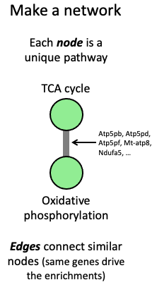
In our implementation, groups of similar pathway enrichments are color-coded, and group labels are inferred from the term names and parents of the pathways in the group. Larger nodes indicate that the pathway was significantly enriched in multiple datasets; thicker edges indicate higher similarity between the pathways.

Best of all, these networks are interactive! Use your cursor to zoom and drag, and hover over nodes and edges to see more information about the underlying data, namely the genes and datasets driving the pathway enrichment.

Minimal example: single tissue

Here we show the interactive network of pathway enrichments corresponding to training-regulated features that are up-regulated in the gastrocnemius in both sexes at the 8-week time point, i.e. SKM-GN:8w_F1_M1.

enrichment_network_vis(tissues="SKM-GN",
                       cluster="8w_F1_M1")
#> Formatting inputs...
#> Subsetting feature-to-gene map...
#> Calculating similarity metric between pairs of enriched pathways...
#> Constructing graph...
#> Elapsed time: 1.864s


# # Equivalently:
# data(GRAPH_PW_ENRICH)
# pw = GRAPH_PW_ENRICH[GRAPH_PW_ENRICH$cluster == "SKM-GN:8w_F1_M1",]
# enrichment_network_vis(pw)

Note that you could run this function with any pathway enrichment results, as long as the columns of pw_enrich_res include “adj_p_value”, “ome”, “tissue”, “intersection”, “computed_p_value”, “term_name”, and “term_id” and the columns of feature_to_gene include “gene_symbol”, “ensembl_gene”. feature$ensembl_gene can be a dummy column if intersection_id_type = "gene_symbol".

Example with multiple tissues

Now let’s examine pathways that are enriched in the same graphical cluster for multiple tissues. For this example, we’ll consider features that are up-regulated in both males and females at the 8-week training time point (8w_F1_M1) in any of our three muscle tissues (heart, gastrocnemius, vastus lateralis).

If we are specifically interested in pathways that are significantly enriched in multiple tissues, we can set multitissue_pathways_only to TRUE. This removes any pathways that are not enriched in more than one tissue (in at least one ome).

enrichment_network_vis(tissues=c("HEART","SKM-GN","SKM-VL"),
                       cluster="8w_F1_M1", 
                       multitissue_pathways_only = TRUE)
#> Formatting inputs...
#> Subsetting feature-to-gene map...
#> Calculating similarity metric between pairs of enriched pathways...
#> Constructing graph...
#> Elapsed time: 1.469s


# # Equivalently:
# pw = GRAPH_PW_ENRICH[grepl(":8w_F1_M1", GRAPH_PW_ENRICH$cluster) & 
#                        GRAPH_PW_ENRICH$tissue %in% c("HEART","SKM-GN","SKM-VL"),]
# enrichment_network_vis(pw, multitissue_pathways_only = TRUE)

Examples with other parameters

Let’s go back to our simple example for input pathway enrichment results.

pw = GRAPH_PW_ENRICH[GRAPH_PW_ENRICH$cluster == "SKM-GN:8w_F1_M1",]

Move or remove group labels

By default, the color-coded node group labels are shown on the left side of the plot. To make it easier to match labels to groups of pathways, we can set the add_group_label_nodes argument to TRUE. If you’re zoomed out, hover over a label to display it in larger font.

enrichment_network_vis(pw, add_group_label_nodes = TRUE)
#> Formatting inputs...
#> Subsetting feature-to-gene map...
#> Calculating similarity metric between pairs of enriched pathways...
#> Constructing graph...
#> Elapsed time: 0.273s


# # Equivalently:
# enrichment_network_vis(tissues="SKM-GN",
#                        cluster="8w_F1_M1",
#                        add_group_label_nodes = TRUE)

You can also remove group labels entirely with label_nodes = FALSE.

enrichment_network_vis(pw, label_nodes = FALSE)
#> Formatting inputs...
#> Subsetting feature-to-gene map...
#> Calculating similarity metric between pairs of enriched pathways...
#> Constructing graph...
#> Elapsed time: 0.267s


# # Equivalently:
# enrichment_network_vis(tissues="SKM-GN",
#                        cluster="8w_F1_M1",
#                        label_nodes = FALSE)

Save similarity scores

Notice that each time we run this function, it takes more than 10 seconds to execute. If you want to play with the parameters of enrichment_network_vis() for the same pathway enrichment results, you can save the pathway similarity scores in a file to avoid re-computing them each time, which is the most computationally expensive step in this function.

similarity_scores_file must specify an RDS file (suffix .rds or .RDS). The first time the function is run with a non-null similarity_scores_file argument, the scores are computed and saved to the given RDS file. Then future calls to this function with similarity_scores_file set to an existing file will load the scores from the file instead of re-computing them. Notice the dramatic difference in elapsed time for these two function calls.

system.time(
  enrichment_network_vis(pw, similarity_scores_file = "/tmp/SKM-GN_8w_F1_M1_scores.RDS", verbose=FALSE)
)
#>    user  system elapsed 
#>   0.292   0.000   0.274
system.time(
  enrichment_network_vis(pw, similarity_scores_file = "/tmp/SKM-GN_8w_F1_M1_scores.RDS", verbose=FALSE)
)
#>    user  system elapsed 
#>   0.197   0.000   0.177

Remove METAB-only enrichments

Since metabolites are not readily mapped to genes, they cannot easily be incorporated into this network where pathway similarity is calculated using the overlap of gene symbols. Therefore, pathway enrichments driven exclusively by metabolites are treated differently. If two pathways are driven exclusively by metabolites, an artificial edge is drawn between them if at least one non-stopword overlaps between the pathway names or parent pathway names. Otherwise, the pathways are represented as singleton nodes. To exclude pathways enriched only by differential metabolites set include_metab_singletons to FALSE.

enrichment_network_vis(pw, include_metab_singletons=FALSE)
#> Formatting inputs...
#> Subsetting feature-to-gene map...
#> Calculating similarity metric between pairs of enriched pathways...
#> Constructing graph...
#> Elapsed time: 0.264s

Export a network to Cytoscape

The output of enrichment_network_vis() is nice for exploration, but it comes short of publication-ready figures. You can export a network to Cytoscape to manually polish it. For this code to work, you need to install the RCy3 R package and have Cytoscape running locally.

library(RCy3)
vn = enrichment_network_vis(pw,
                            title = "SKM-GN:8w_F1_M1",
                            return_graph_for_cytoscape = TRUE) 
cytoscapePing()
createNetworkFromIgraph(vn, new.title='gastroc-8w-both-up')

Once you’ve imported the network into Cytoscape, you can import the style sheet found here and follow these instructions to quickly make beautiful network with nodes colored by either tissue or ome. For example: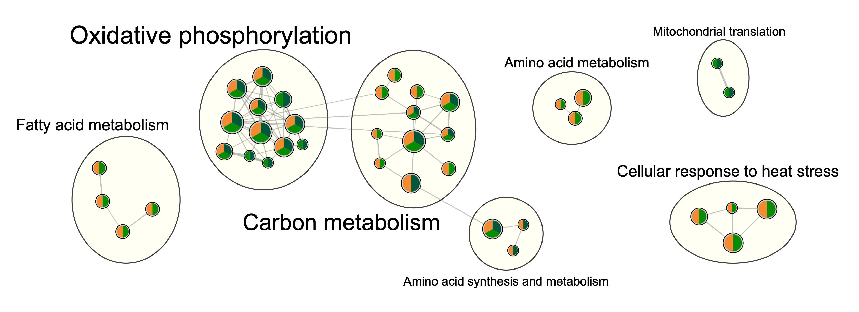

Printing networks within a loop

Rendering visNetwork objects within a loop has some known challenges. See solutions here.

Getting help

For questions, bug reporting, and feature requests for this package, please submit a new issue and include as many details as possible.

If the concern is related to data provided in the MotrpacRatTraining6moData package, please submit an issue here instead.

Acknowledgements

MoTrPAC is supported by the National Institutes of Health (NIH) Common Fund through cooperative agreements managed by the National Institute of Diabetes and Digestive and Kidney Diseases (NIDDK), National Institute of Arthritis and Musculoskeletal Diseases (NIAMS), and National Institute on Aging (NIA).

Session Info

sessionInfo()
#> R version 4.4.1 (2024-06-14)
#> Platform: x86_64-pc-linux-gnu
#> Running under: Ubuntu 22.04.5 LTS
#> 
#> Matrix products: default
#> BLAS:   /usr/lib/x86_64-linux-gnu/openblas-pthread/libblas.so.3 
#> LAPACK: /usr/lib/x86_64-linux-gnu/openblas-pthread/libopenblasp-r0.3.20.so;  LAPACK version 3.10.0
#> 
#> locale:
#>  [1] LC_CTYPE=C.UTF-8       LC_NUMERIC=C           LC_TIME=C.UTF-8       
#>  [4] LC_COLLATE=C.UTF-8     LC_MONETARY=C.UTF-8    LC_MESSAGES=C.UTF-8   
#>  [7] LC_PAPER=C.UTF-8       LC_NAME=C              LC_ADDRESS=C          
#> [10] LC_TELEPHONE=C         LC_MEASUREMENT=C.UTF-8 LC_IDENTIFICATION=C   
#> 
#> time zone: UTC
#> tzcode source: system (glibc)
#> 
#> attached base packages:
#> [1] stats     graphics  grDevices utils     datasets  methods   base     
#> 
#> other attached packages:
#> [1] foreach_1.5.2                   gprofiler2_0.2.3               
#> [3] repfdr_1.2.3                    MotrpacRatTraining6mo_1.6.6    
#> [5] MotrpacRatTraining6moData_2.0.0
#> 
#> loaded via a namespace (and not attached):
#>   [1] bitops_1.0-8            Rdpack_2.6.1            mnormt_2.1.1           
#>   [4] gridExtra_2.3           fdrtool_1.2.18          sandwich_3.1-1         
#>   [7] rlang_1.1.4             magrittr_2.0.3          multcomp_1.4-26        
#>  [10] qqconf_1.3.2            compiler_4.4.1          png_0.1-8              
#>  [13] systemfonts_1.1.0       vctrs_0.6.5             crayon_1.5.3           
#>  [16] pkgconfig_2.0.3         fastmap_1.2.0           XVector_0.44.0         
#>  [19] labeling_0.4.3          ggraph_2.2.1            utf8_1.2.4             
#>  [22] r2r_0.1.1               rmarkdown_2.28          UCSC.utils_1.0.0       
#>  [25] ragg_1.3.3              purrr_1.0.2             xfun_0.47              
#>  [28] zlibbioc_1.50.0         cachem_1.1.0            GenomeInfoDb_1.40.1    
#>  [31] jsonlite_1.8.9          highr_0.11              tweenr_2.0.3           
#>  [34] R6_2.5.1                bslib_0.8.0             RColorBrewer_1.1-3     
#>  [37] limma_3.60.4            mutoss_0.1-13           jquerylib_0.1.4        
#>  [40] numDeriv_2016.8-1.1     iterators_1.0.14        Rcpp_1.0.13            
#>  [43] knitr_1.48              zoo_1.8-12              IRanges_2.38.1         
#>  [46] Matrix_1.7-0            splines_4.4.1           igraph_2.0.3           
#>  [49] tidyselect_1.2.1        yaml_2.3.10             viridis_0.6.5          
#>  [52] codetools_0.2-20        plyr_1.8.9              lattice_0.22-6         
#>  [55] tibble_3.2.1            KEGGREST_1.44.1         Biobase_2.64.0         
#>  [58] withr_3.0.1             evaluate_1.0.0          desc_1.4.3             
#>  [61] survival_3.6-4          polyclip_1.10-7         Biostrings_2.72.1      
#>  [64] IHW_1.32.0              pillar_1.9.0            stats4_4.4.1           
#>  [67] lpsymphony_1.32.0       sn_2.1.1                plotly_4.10.4          
#>  [70] generics_0.1.3          RCurl_1.98-1.16         mathjaxr_1.6-0         
#>  [73] S4Vectors_0.42.1        ggplot2_3.5.1           munsell_0.5.1          
#>  [76] scales_1.3.0            TFisher_0.2.0           glue_1.7.0             
#>  [79] slam_0.1-53             lazyeval_0.2.2          tools_4.4.1            
#>  [82] metap_1.11              data.table_1.16.0       locfit_1.5-9.10        
#>  [85] fs_1.6.4                visNetwork_2.1.2        mvtnorm_1.3-1          
#>  [88] graphlayouts_1.2.0      tidygraph_1.3.1         grid_4.4.1             
#>  [91] plotrix_3.8-6           tidyr_1.3.1             rbibutils_2.2.16       
#>  [94] edgeR_4.2.1             colorspace_2.1-1        GenomeInfoDbData_1.2.12
#>  [97] ggforce_0.4.2           cli_3.6.3               textshaping_0.4.0      
#> [100] fansi_1.0.6             viridisLite_0.4.2       dplyr_1.1.4            
#> [103] gtable_0.3.5            sass_0.4.9              digest_0.6.37          
#> [106] BiocGenerics_0.50.0     ggrepel_0.9.6           TH.data_1.1-2          
#> [109] htmlwidgets_1.6.4       farver_2.1.2            memoise_2.0.1          
#> [112] htmltools_0.5.8.1       pkgdown_2.1.1           multtest_2.60.0        
#> [115] lifecycle_1.0.4         httr_1.4.7              statmod_1.5.0          
#> [118] FELLA_1.24.0            MASS_7.3-60.2

Introduction

About this package

About MoTrPAC

Setup

Study design

Tissue and assay abbreviations

Tissues

Assays/omes

Data in MotrpacRatTraining6moData

Differential analysis

Bayesian graphical clustering

Summary

(Re-)run repfdr to determine states

Explore graphical clustering results

Plot graph of differential features

Pathway enrichment of clusters

Approach

Enrichment with standard PWs

Enrichment with custom PWs

Simple enrichment with single gene set

Visualization of PW enrichments

Approach

Minimal example: single tissue

Example with multiple tissues

Examples with other parameters

Move or remove group labels

Save similarity scores

Remove METAB-only enrichments

Export a network to Cytoscape

Printing networks within a loop

Getting help

Acknowledgements

Session Info

(Re-)run `repfdr` to determine states