Plots of Top FGSEA Terms from Male vs. Female Comparisons

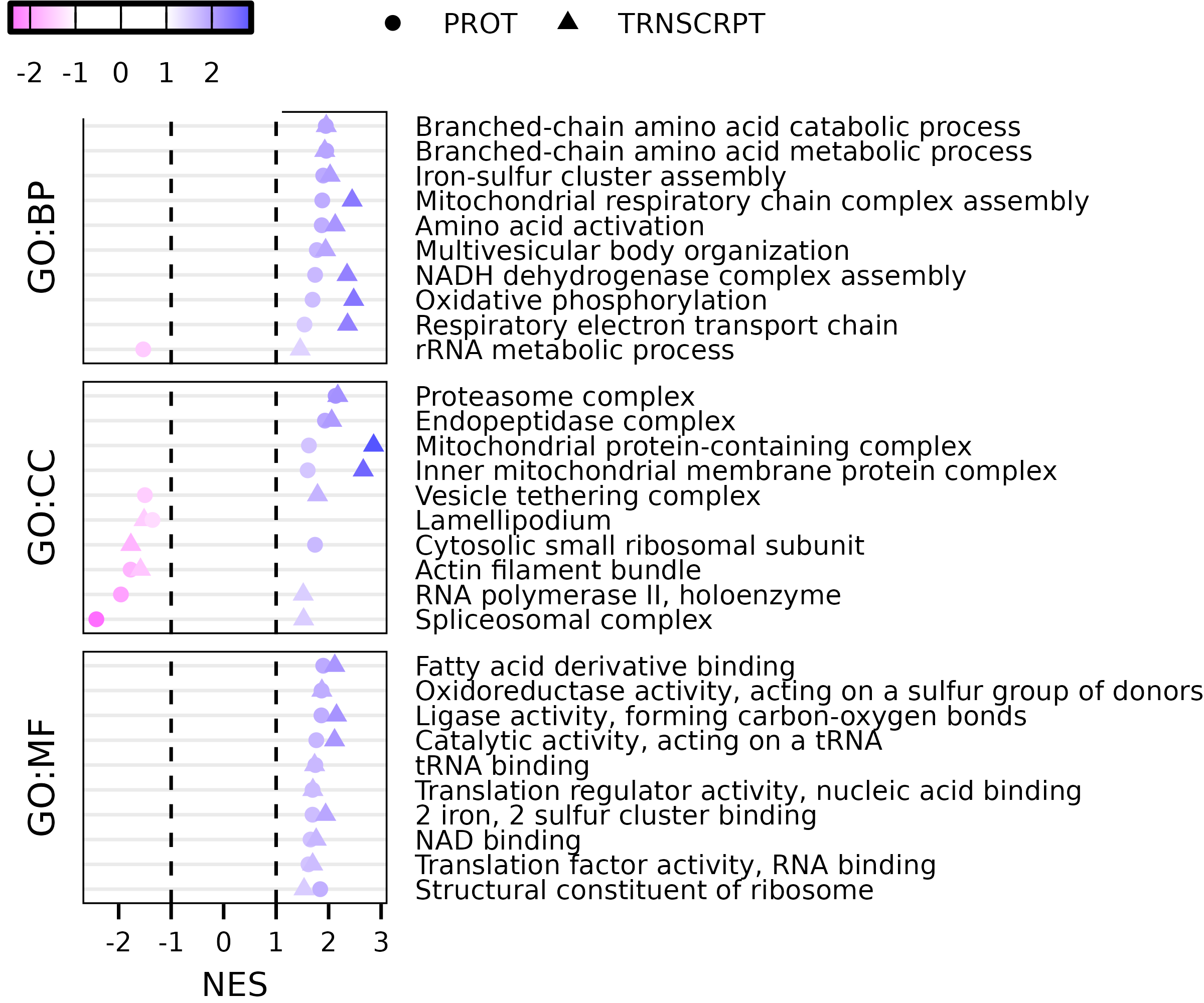
This article generates scatterplots of the top FGSEA terms from the male vs. female comparisons (Fig. 2B, C).

library(MotrpacRatTraining6moWATData)
library(MotrpacRatTraining6moWAT)
library(dplyr)
library(purrr)
library(tidyr)
library(data.table)
library(ggplot2)
library(grid)

save_plots <- dir.exists(paths = file.path("..", "..", "plots"))

omes <- c("PROT", "TRNSCRPT")

res <- lapply(omes, function(ome) {
  file <- paste0(ome, "_FGSEA")
  fgsea_res <- get(file)

  pluck(fgsea_res, "MvF_SED") %>%
    mutate(ome = ome)
})

common_sets <- intersect(res[[1]]$pathway, res[[2]]$pathway)

res_df <- rbindlist(res) %>%
  dplyr::select(ome, contrast, gs_subcat, pathway, 
                gs_description, padj, NES) %>%
  pivot_wider(id_cols = c(contrast:gs_description),
              names_from = ome,
              values_from = c(padj, NES),
              names_sep = ".") %>%
  filter(!(is.na(NES.PROT) | is.na(NES.TRNSCRPT))) %>%
  mutate(both_signif = padj.PROT < 0.05 & padj.TRNSCRPT < 0.05,
         quadrant = case_when(NES.PROT > 0 & NES.TRNSCRPT > 0 ~ "Q1",
                              NES.PROT < 0 & NES.TRNSCRPT > 0 ~ "Q2",
                              NES.PROT < 0 & NES.TRNSCRPT < 0 ~ "Q3",
                              NES.PROT > 0 & NES.TRNSCRPT < 0 ~ "Q4")) %>%
  arrange(both_signif)

top_terms <- res_df %>%
  filter(both_signif) %>%
  dplyr::select(-both_signif) %>%
  group_by(pathway, gs_subcat, quadrant, gs_description) %>%
  rowwise() %>%
  mutate(NES_mean = mean(abs(c(NES.PROT, NES.TRNSCRPT)))) %>%
  ungroup() %>%
  group_by(gs_subcat) %>%
  arrange(-NES_mean) %>%
  mutate(not_Q1 = sum(quadrant != "Q1"),
         n = 10 - not_Q1) %>%
  group_by(gs_subcat, quadrant) %>%
  mutate(idx = 1:n()) %>%
  filter((idx <= not_Q1 & quadrant != "Q1") |
           (idx <= n & quadrant == "Q1")) %>%
  pull(pathway)

p1 <- ggplot(res_df) +
  geom_vline(xintercept = 0, lty = "dashed",
             color = "black", linewidth = 0.3) +
  geom_hline(yintercept = 0, lty = "dashed",
             color = "black", linewidth = 0.3) +
  geom_point(aes(x = NES.PROT, y = NES.TRNSCRPT,
                 color = both_signif),
             size = 0.8, shape = 16, alpha = 0.85) +
  facet_grid(gs_subcat ~ ., space = "free_y") +
  labs(x = "NES: PROT", y = "NES: TRNSCRPT") +
  scale_color_manual(name = NULL,
                     values = c("black", "grey"),
                     labels = c("Significantly enriched in both -omes"),
                     breaks = c(TRUE), na.value = "grey") +
  theme_pub() +
  theme(legend.position = "top",
        legend.margin = margin(t = 0, b = -5),
        legend.box.margin = margin(b = -5, t = -5),
        axis.line = element_line(color = NA),
        panel.border = element_rect(color = "black", fill = NA),
        strip.background = element_blank())

p1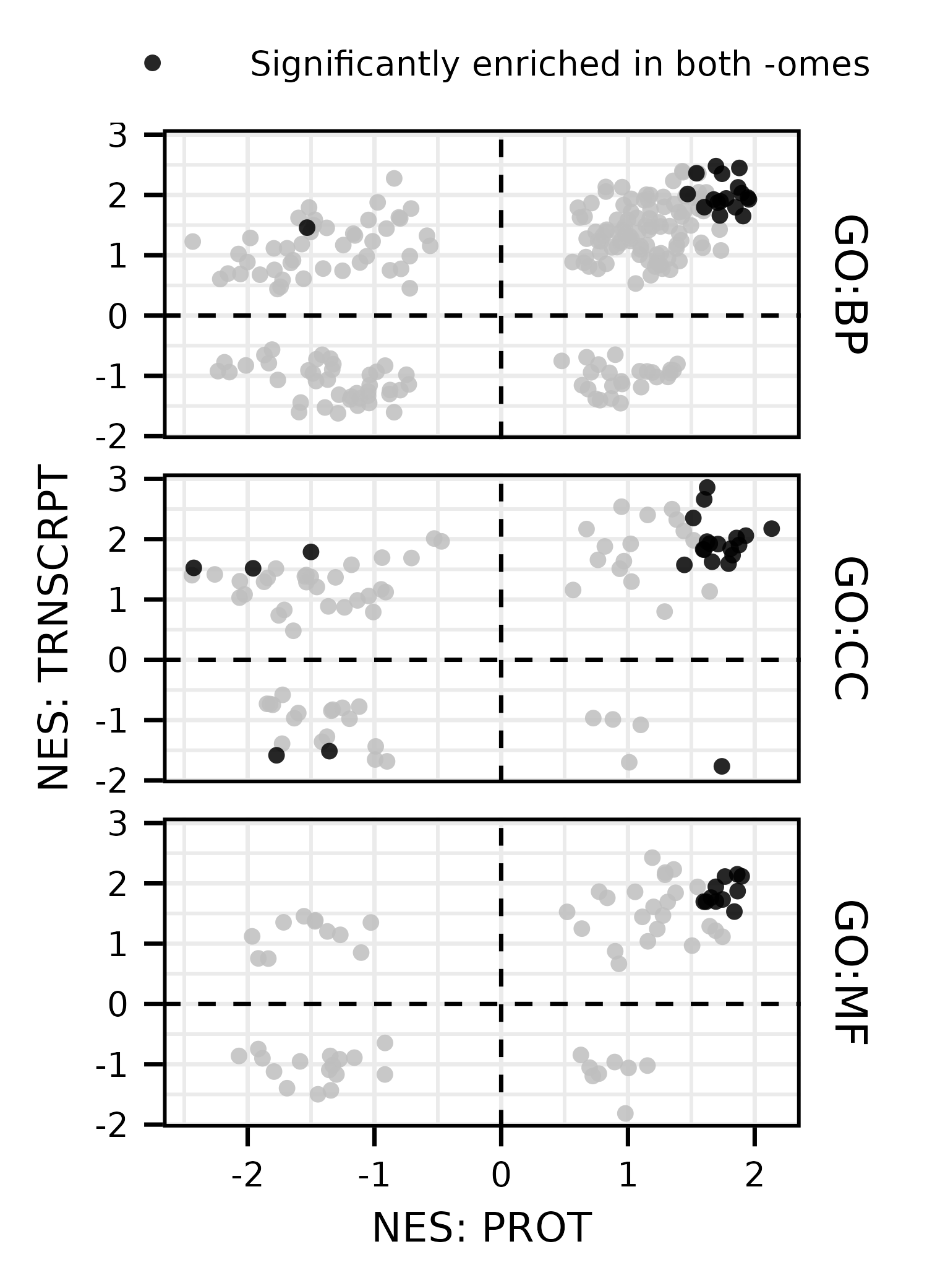

ggsave(file.path("..", "..", "plots", "FGSEA_NES_scatterplot.pdf"), p1,
       height = 2.6, width = 1.9, family = "ArialMT")

p2 <- res_df %>%
  filter(pathway %in% top_terms) %>%
  pivot_longer(cols = c(contains("NES"), contains("padj"))) %>%
  separate(col = name, into = c("measure", "ome"),
           sep = "\\.", remove = TRUE) %>%
  pivot_wider(names_from = measure,
              values_from = value) %>%
  arrange(NES) %>%
  mutate(gs_description = factor(gs_description,
                                 levels = unique(gs_description))) %>%
  ggplot() +
  geom_vline(xintercept = c(-1, 1), color = "black",
             lty = "dashed", linewidth = 0.3) +
  geom_point(aes(x = NES, y = gs_description,
                 shape = ome, color = NES),
             size = 1) +
  facet_grid(gs_subcat ~ ., scales = "free_y",
             switch = "y", space = "free_y") +
  scale_y_discrete(name = NULL,
                   position = "right") +
  scale_color_gradientn(colors = c("#ff6eff", rep("white", 2), "#5555ff"),
                        values = scales::rescale(c(-2.5, -1, 1, 2.9))) +
  scale_shape_manual(name = NULL, values = 16:17) +
  guides(
    color = guide_colorbar(barwidth = unit(0.6, "in"),
                           barheight = unit(0.07, "in"),
                           frame.colour = "black",
                           ticks.colour = "black", order = 1),
    shape = guide_legend(title =  NULL, order = 2,
                         keyheight = unit(7, "pt"),
                         keywidth = unit(7, "pt"))) +
  theme_bw() +
  theme(text = element_text(size = 6, color = "black"),
        axis.text = element_text(color = "black"),
        axis.title = element_text(color = "black"),
        axis.ticks.y = element_blank(),
        axis.ticks.x = element_line(color = "black", linewidth = 0.3),
        axis.title.y = element_text(margin = margin(r = 10, unit = "pt")),
        strip.background = element_blank(),
        strip.text = element_text(size = 6.5, color = "black"),
        panel.spacing.y = unit(3, "pt"),
        panel.border = element_rect(fill = NA, color = "black",
                                    linewidth = 0.3),
        plot.margin = margin(t = 20, unit = "pt"),
        legend.position = c(0.85, 1.1),
        legend.direction = "horizontal",
        legend.box = "horizontal",
        legend.box.margin = margin(b = -5, unit = "pt"),
        legend.title = element_text(size = 5.5,
                                    color = "black"),
        legend.text = element_text(size = 5,
                                   color = "black"),
        panel.grid = element_blank(),
        panel.grid.major.y = element_line(linewidth = 0.3, color = "grey92"))

p2

ggsave(file.path("..", "..", "plots", "FGSEA_NES_scatterplot_terms.pdf"), p2,
       height = 2.5, width = 3, family = "ArialMT")

Tyler Sagendorf

01 May, 2024