Statistical analyses of plasma clinical analytes
Tyler Sagendorf
01 May, 2024
Source:vignettes/ANALYTES_STATS.Rmd
ANALYTES_STATS.Rmd
# Required packages
library(MotrpacRatTrainingPhysiologyData)
library(ggplot2)
library(dplyr)
library(emmeans)
library(tibble)
library(tidyr)
library(purrr)
library(latex2exp)
theme_set(theme_bw()) # base plot theme
Regression Models
Since clinical analytes are strictly positive, we will check the mean–variance relationship with code from Dunn and Smyth[1] (pg. 429–430) and fit an appropriate log-link generalized linear model (GLM). This allows us to back-transform the means without introducing bias, unlike when the response is transformed. Also, the log-link allows us to test ratios between means, rather than their absolute differences.
If there are obvious problems with the model diagnostic plots, or the mean–variance relationship does not correspond to an exponential family distribution, we will include inverse group variances as weights in a log-link Gaussian GLM. Finally, we will remove insignificant predictors to achieve model parsimony based on ANOVA F-tests.
Corticosterone
Corticosterone (ng/mL).
# Plot points
ggplot(ANALYTES, aes(x = group, y = corticosterone)) +
  geom_point(position = position_jitter(width = 0.1, height = 0),
             na.rm = TRUE) +
  facet_wrap(~ age + sex, nrow = 1) +
  theme(axis.text.x = element_text(angle = 90, hjust = 1, vjust = 0.5))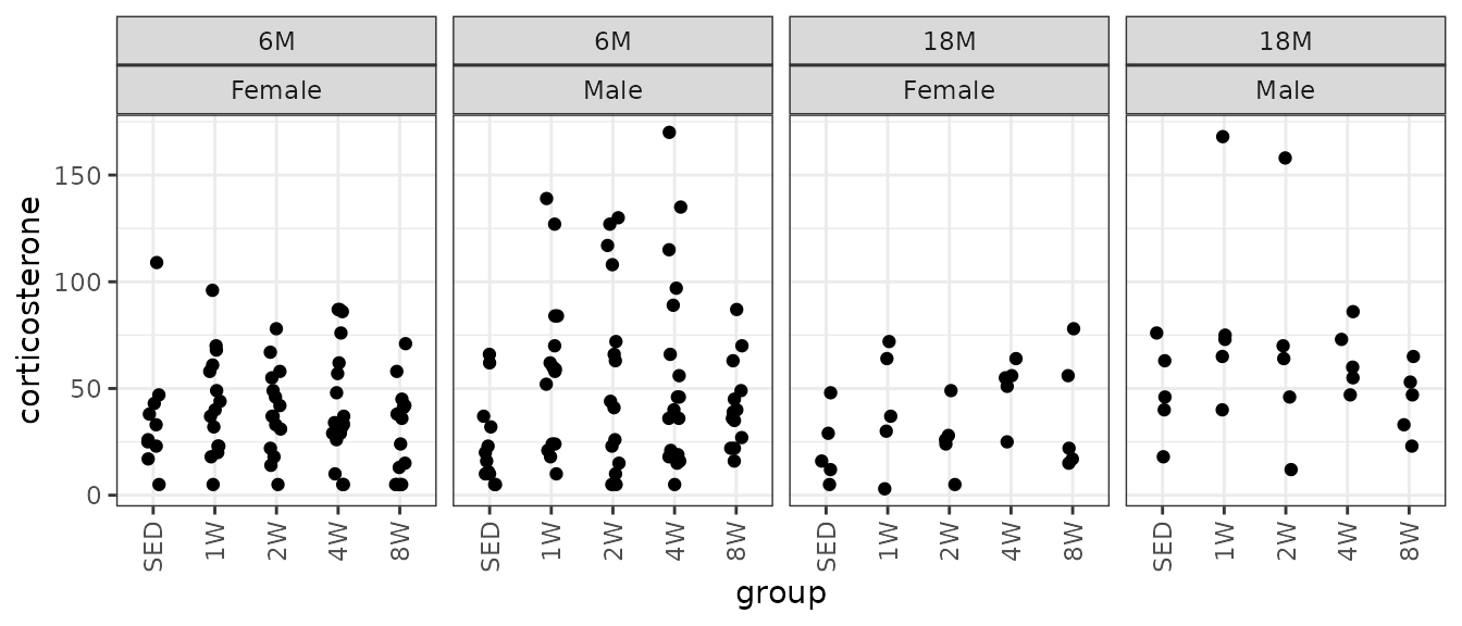
We will check the mean-variance relationship.
mv <- ANALYTES %>%
  group_by(sex, group, age) %>%
  summarise(mn = mean(corticosterone, na.rm = TRUE),
            vr = var(corticosterone, na.rm = TRUE),
            .groups = "keep")

fit.mv <- lm(log(vr) ~ log(mn), data = mv)
coef(fit.mv)
#> (Intercept)     log(mn)
#>    1.258480    1.382773
plot(log(vr) ~ log(mn), data = mv, las = 1, pch = 19,
     xlab = "log(group means)", ylab = "log(group variances)")
abline(coef(fit.mv), lwd = 2)
The slope is closer to 1 than 2, so we will use a quasi-Poisson distribution.
fit.cort <- glm(corticosterone ~ age * sex * group,
                family = quasipoisson("log"),
                data = ANALYTES)
plot_lm(fit.cort)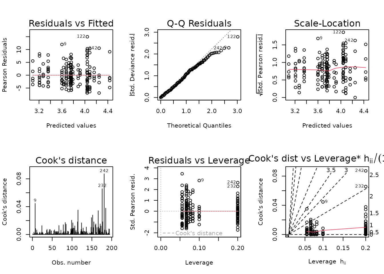
The model seems to be a poor fit. We will try a log-link Gaussian GLM with inverse group variance weights.
wt.cort <- ANALYTES %>%
  group_by(age, sex, group) %>%
  mutate(1 / var(corticosterone, na.rm = TRUE)) %>%
  pull(-1)

fit.cort <- update(fit.cort, family = gaussian("log"),
                   weights = wt.cort)
plot_lm(fit.cort)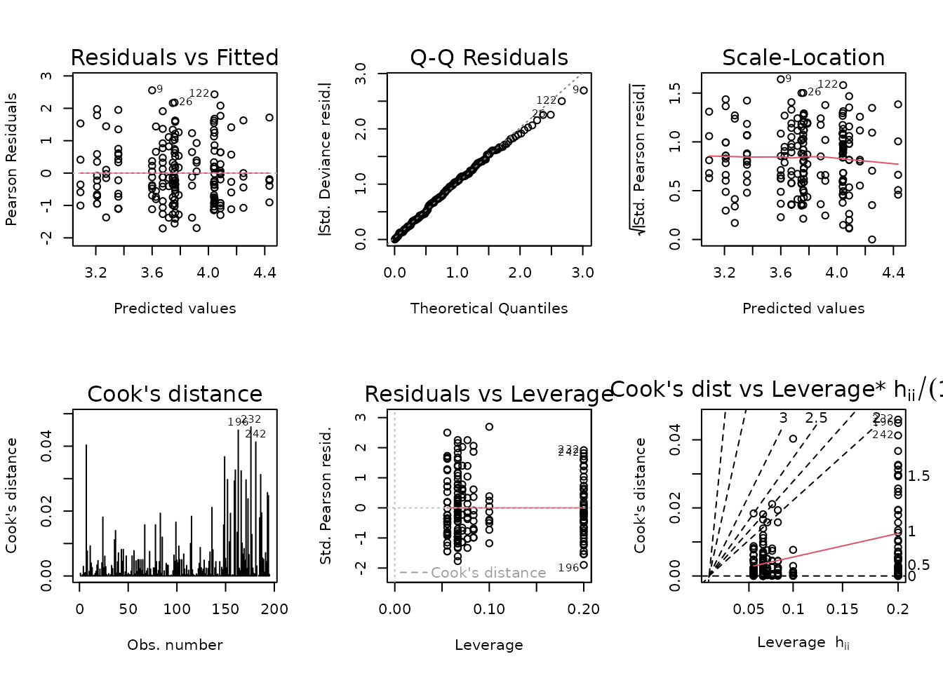
The diagnostic plots seem mostly fine, though the left tail of the QQ-plot seems light. We will try to simplify the model to improve the model fit.
anova(fit.cort, test = "F")
#> Analysis of Deviance Table
#>
#> Model: gaussian, link: log
#>
#> Response: corticosterone
#>
#> Terms added sequentially (first to last)
#>
#>
#>               Df Deviance Resid. Df Resid. Dev      F    Pr(>F)
#> NULL                            194     224.85
#> age            1   1.3691       193     223.48 1.3690  0.243578
#> sex            1   8.4384       192     215.04 8.4380  0.004149 **
#> group          4  28.2334       188     186.81 7.0580 2.727e-05 ***
#> age:sex        1   1.4328       187     185.38 1.4328  0.232932
#> age:group      4   2.6398       183     182.74 0.6599  0.620660
#> sex:group      4   2.0953       179     180.64 0.5238  0.718373
#> age:sex:group  4   5.6396       175     175.00 1.4098  0.232623
#> ---
#> Signif. codes:  0 '***' 0.001 '**' 0.01 '*' 0.05 '.' 0.1 ' ' 1
fit.cort.1 <- update(fit.cort, formula = . ~ sex + group)
anova(fit.cort.1, fit.cort, test = "F")
#> Analysis of Deviance Table
#>
#> Model 1: corticosterone ~ sex + group
#> Model 2: corticosterone ~ age * sex * group
#>   Resid. Df Resid. Dev Df Deviance      F Pr(>F)
#> 1       189      187.4
#> 2       175      175.0 14     12.4 0.8857 0.5754
There is no significant difference between the full model and the one with only sex and group as predictors.
fit.cort <- fit.cort.1
plot_lm(fit.cort)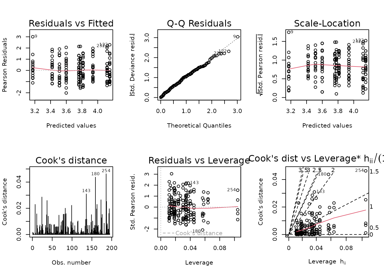
summary(fit.cort)
#>
#> Call:
#> glm(formula = corticosterone ~ sex + group, family = gaussian("log"),
#>     data = ANALYTES, weights = wt.cort)
#>
#> Coefficients:
#>             Estimate Std. Error t value Pr(>|t|)
#> (Intercept)  3.17354    0.14297  22.197  < 2e-16 ***
#> sexMale      0.33925    0.08581   3.953 0.000109 ***
#> group1W      0.60556    0.16273   3.721 0.000261 ***
#> group2W      0.42548    0.16805   2.532 0.012157 *
#> group4W      0.63936    0.14661   4.361 2.13e-05 ***
#> group8W      0.24682    0.15715   1.571 0.117949
#> ---
#> Signif. codes:  0 '***' 0.001 '**' 0.01 '*' 0.05 '.' 0.1 ' ' 1
#>
#> (Dispersion parameter for gaussian family taken to be 0.9915343)
#>
#>     Null deviance: 224.85  on 194  degrees of freedom
#> Residual deviance: 187.40  on 189  degrees of freedom
#>   (87 observations deleted due to missingness)
#> AIC: 1845.4
#>
#> Number of Fisher Scoring iterations: 6
Glucagon
Glucagon (pM).
# Plot points
ggplot(ANALYTES, aes(x = group, y = glucagon)) +
  geom_point(position = position_jitter(width = 0.1, height = 0),
             na.rm = TRUE) +
  facet_wrap(~ age + sex, nrow = 1) +
  theme(axis.text.x = element_text(angle = 90, hjust = 1, vjust = 0.5))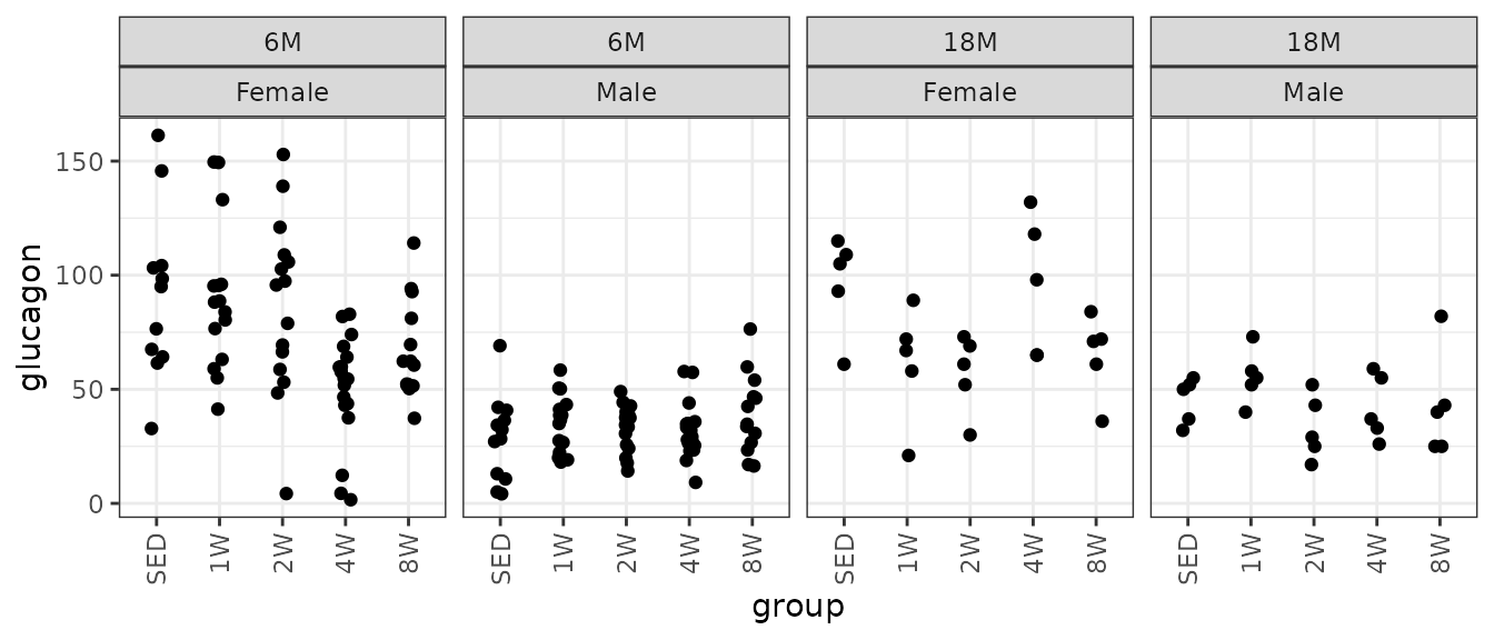
We will check the mean-variance relationship.
mv <- ANALYTES %>%
  group_by(sex, group, age) %>%
  summarise(mn = mean(glucagon, na.rm = TRUE),
            vr = var(glucagon, na.rm = TRUE))

fit.mv <- lm(log(vr) ~ log(mn), data = mv)
coef(fit.mv)
#> (Intercept)     log(mn)
#>  -0.1011426   1.5066221
plot(log(vr) ~ log(mn), data = mv, las = 1, pch = 19,
     xlab = "log(group means)", ylab = "log(group variances)")
abline(coef(fit.mv), lwd = 2)
The slope suggests a variance function approximately of the form \(V(\mu) = \mu^{1.5}\)). This is intermediate between the Poisson and gamma distributions. We will fit a quasi-Poisson GLM since we are not dealing with count data.
fit.glucagon <- glm(glucagon ~ age * sex * group,
                    family = quasipoisson("log"),
                    data = ANALYTES)
plot_lm(fit.glucagon)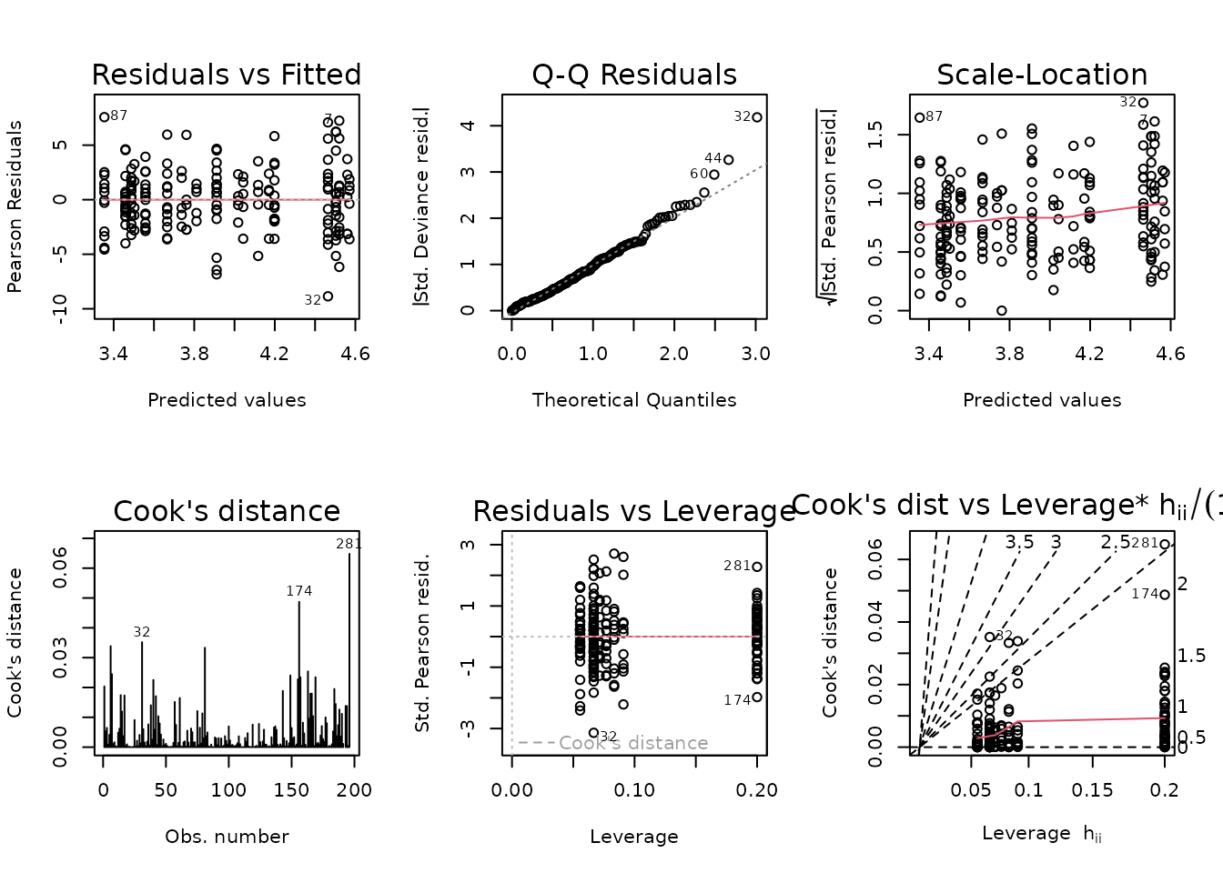
The diagnostic plots look fine. We will try to simplify the model.
anova(fit.glucagon, test = "F")
#> Analysis of Deviance Table
#>
#> Model: quasipoisson, link: log
#>
#> Response: glucagon
#>
#> Terms added sequentially (first to last)
#>
#>
#>               Df Deviance Resid. Df Resid. Dev        F    Pr(>F)
#> NULL                            195     3517.0
#> age            1    16.90       194     3500.1   1.9815  0.160999
#> sex            1  1381.68       193     2118.4 162.0164 < 2.2e-16 ***
#> group          4   124.07       189     1994.4   3.6371  0.007115 **
#> age:sex        1    37.04       188     1957.3   4.3428  0.038610 *
#> age:group      4   151.57       184     1805.8   4.4432  0.001910 **
#> sex:group      4    84.87       180     1720.9   2.4880  0.045129 *
#> age:sex:group  4    84.33       176     1636.6   2.4723  0.046262 *
#> ---
#> Signif. codes:  0 '***' 0.001 '**' 0.01 '*' 0.05 '.' 0.1 ' ' 1
The 3-way intersection is significant, so we will not remove any terms.
summary(fit.glucagon)
#>
#> Call:
#> glm(formula = glucagon ~ age * sex * group, family = quasipoisson("log"),
#>     data = ANALYTES)
#>
#> Coefficients:
#>                        Estimate Std. Error t value Pr(>|t|)
#> (Intercept)             4.52021    0.09187  49.202  < 2e-16 ***
#> age18M                  0.05037    0.16154   0.312  0.75555
#> sexMale                -1.16651    0.18242  -6.395 1.40e-09 ***
#> group1W                -0.01663    0.12138  -0.137  0.89121
#> group2W                -0.05614    0.12242  -0.459  0.64711
#> group4W                -0.60907    0.13388  -4.549 9.99e-06 ***
#> group8W                -0.32204    0.13263  -2.428  0.01619 *
#> age18M:sexMale          0.40703    0.29777   1.367  0.17340
#> age18M:group1W         -0.43654    0.24529  -1.780  0.07685 .
#> age18M:group2W         -0.47139    0.25013  -1.885  0.06114 .
#> age18M:group4W          0.59867    0.23113   2.590  0.01040 *
#> age18M:group8W         -0.07724    0.24813  -0.311  0.75597
#> sexMale:group1W         0.22056    0.23617   0.934  0.35164
#> sexMale:group2W         0.19002    0.23918   0.794  0.42799
#> sexMale:group4W         0.71379    0.24016   2.972  0.00337 **
#> sexMale:group8W         0.63407    0.24333   2.606  0.00995 **
#> age18M:sexMale:group1W  0.43970    0.41185   1.068  0.28716
#> age18M:sexMale:group2W  0.02896    0.44033   0.066  0.94764
#> age18M:sexMale:group4W -0.77681    0.41415  -1.876  0.06235 .
#> age18M:sexMale:group8W -0.28469    0.42496  -0.670  0.50378
#> ---
#> Signif. codes:  0 '***' 0.001 '**' 0.01 '*' 0.05 '.' 0.1 ' ' 1
#>
#> (Dispersion parameter for quasipoisson family taken to be 8.528022)
#>
#>     Null deviance: 3517.0  on 195  degrees of freedom
#> Residual deviance: 1636.6  on 176  degrees of freedom
#>   (86 observations deleted due to missingness)
#> AIC: NA
#>
#> Number of Fisher Scoring iterations: 4
Glucose
Glucose (mg/dL).
# Plot points
ggplot(ANALYTES, aes(x = group, y = glucose)) +
  geom_point(position = position_jitter(width = 0.1, height = 0),
             na.rm = TRUE) +
  facet_wrap(~ age + sex, nrow = 1) +
  theme(axis.text.x = element_text(angle = 90, hjust = 1, vjust = 0.5))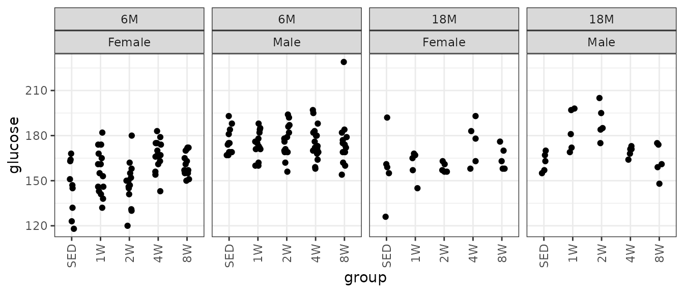
There are several outlying values in the 18M SED female and 6M 8W male groups. We will check the mean-variance relationship.
mv <- ANALYTES %>%
  group_by(sex, group, age) %>%
  summarise(mn = mean(glucose, na.rm = TRUE),
            vr = var(glucose, na.rm = TRUE))

fit.mv <- lm(log(vr) ~ log(mn), data = mv)
coef(fit.mv)
#> (Intercept)     log(mn)
#>   9.2366703  -0.8963349
plot(log(vr) ~ log(mn), data = mv, las = 1, pch = 19,
     xlab = "log(group means)", ylab = "log(group variances)")
abline(coef(fit.mv), lwd = 2)
The slope indicates a slightly decreasing mean-variance trend, though some groups have lower variances than expected, based on the others. We will fit a log-link Gaussian GLM with inverse group variance weights.
wt.glucose <- ANALYTES %>%
  group_by(age, sex, group) %>%
  mutate(1 / var(glucose, na.rm = TRUE)) %>%
  pull(-1)

fit.glucose <- glm(glucose ~ age * sex * group,
                   family = gaussian("log"),
                   weights = wt.glucose,
                   data = ANALYTES)
plot_lm(fit.glucose)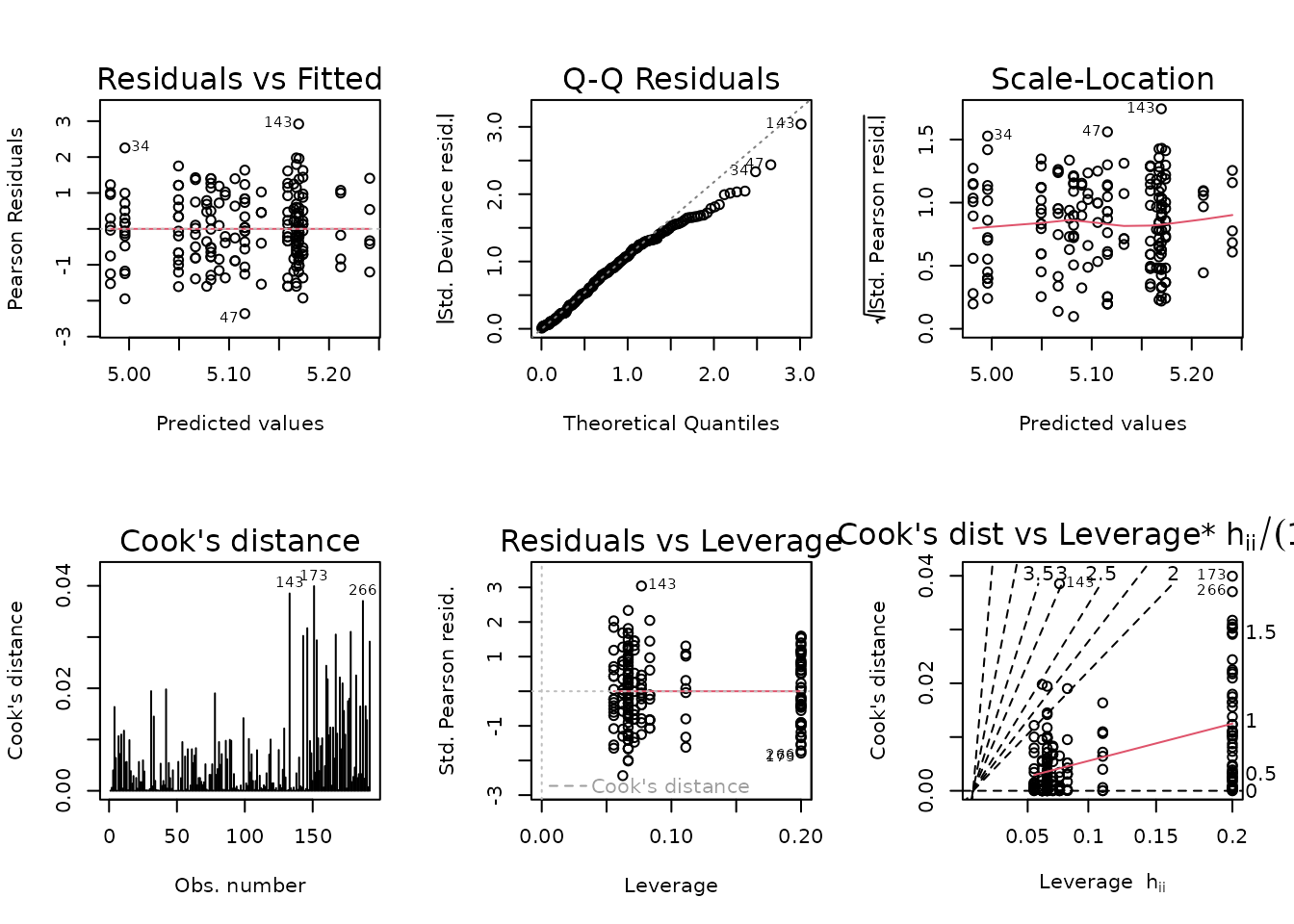
The diagnostic plots look fine. We will try to simplify the model.
anova(fit.glucose, test = "F")
#> Analysis of Deviance Table
#>
#> Model: gaussian, link: log
#>
#> Response: glucose
#>
#> Terms added sequentially (first to last)
#>
#>
#>               Df Deviance Resid. Df Resid. Dev       F    Pr(>F)
#> NULL                            191     344.83
#> age            1    7.690       190     337.14  7.6904  0.006164 **
#> sex            1   98.025       189     239.11 98.0247 < 2.2e-16 ***
#> group          4    5.258       185     233.85  1.3146  0.266475
#> age:sex        1   10.226       184     223.63 10.2265  0.001648 **
#> age:group      4    8.622       180     215.01  2.1554  0.076077 .
#> sex:group      4   36.174       176     178.83  9.0436 1.184e-06 ***
#> age:sex:group  4    6.832       172     172.00  1.7080  0.150361
#> ---
#> Signif. codes:  0 '***' 0.001 '**' 0.01 '*' 0.05 '.' 0.1 ' ' 1
fit.glucose.1 <- update(fit.glucose,
                        formula = . ~ sex * (age + group))
fit.glucose.2 <- update(fit.glucose,
                        formula = . ~ (sex + age + group) ^ 2)
anova(fit.glucose.1, fit.glucose.2, fit.glucose, test = "F")
#> Analysis of Deviance Table
#>
#> Model 1: glucose ~ sex + age + group + sex:age + sex:group
#> Model 2: glucose ~ sex + age + group + sex:age + sex:group + age:group
#> Model 3: glucose ~ age * sex * group
#>   Resid. Df Resid. Dev Df Deviance      F   Pr(>F)
#> 1       180     194.28
#> 2       176     178.83  4  15.4500 3.8625 0.004956 **
#> 3       172     172.00  4   6.8321 1.7080 0.150361
#> ---
#> Signif. codes:  0 '***' 0.001 '**' 0.01 '*' 0.05 '.' 0.1 ' ' 1
We will use the model with all 2-way interactions.
fit.glucose <- fit.glucose.2
plot_lm(fit.glucose)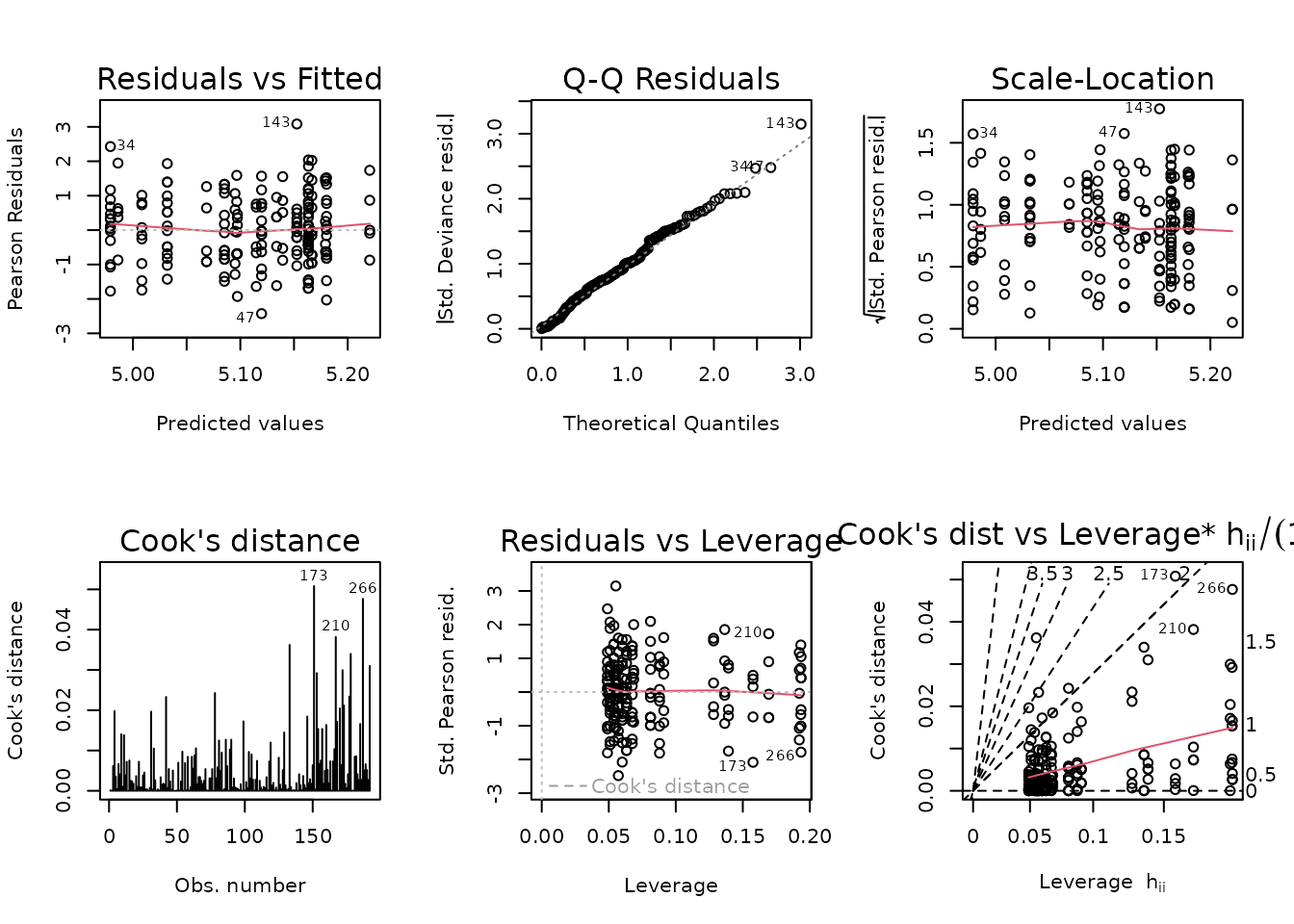
summary(fit.glucose)
#>
#> Call:
#> glm(formula = glucose ~ sex + age + group + sex:age + sex:group +
#>     age:group, family = gaussian("log"), data = ANALYTES, weights = wt.glucose)
#>
#> Coefficients:
#>                 Estimate Std. Error t value Pr(>|t|)
#> (Intercept)      5.00831    0.03622 138.284  < 2e-16 ***
#> sexMale          0.15834    0.03779   4.190 4.41e-05 ***
#> age18M          -0.02227    0.03032  -0.734 0.463756
#> group1W          0.02367    0.04213   0.562 0.574959
#> group2W         -0.02930    0.04134  -0.709 0.479400
#> group4W          0.11147    0.03865   2.884 0.004413 **
#> group8W          0.07689    0.03816   2.015 0.045419 *
#> sexMale:age18M  -0.04931    0.02245  -2.197 0.029335 *
#> sexMale:group1W -0.02699    0.04432  -0.609 0.543278
#> sexMale:group2W  0.04294    0.04325   0.993 0.322196
#> sexMale:group4W -0.11469    0.04175  -2.747 0.006633 **
#> sexMale:group8W -0.09089    0.04480  -2.029 0.043964 *
#> age18M:group1W   0.08756    0.03543   2.471 0.014416 *
#> age18M:group2W   0.11180    0.03234   3.457 0.000686 ***
#> age18M:group4W   0.04195    0.02733   1.535 0.126644
#> age18M:group8W   0.03374    0.03436   0.982 0.327500
#> ---
#> Signif. codes:  0 '***' 0.001 '**' 0.01 '*' 0.05 '.' 0.1 ' ' 1
#>
#> (Dispersion parameter for gaussian family taken to be 1.016093)
#>
#>     Null deviance: 344.83  on 191  degrees of freedom
#> Residual deviance: 178.83  on 176  degrees of freedom
#>   (90 observations deleted due to missingness)
#> AIC: 1478
#>
#> Number of Fisher Scoring iterations: 4
Glycerol
Glycerol (mg/dL).
# Plot points
ggplot(ANALYTES, aes(x = group, y = glycerol)) +
  geom_point(position = position_jitter(width = 0.1, height = 0),
             na.rm = TRUE) +
  facet_wrap(~ age + sex, nrow = 1) +
  theme(axis.text.x = element_text(angle = 90, hjust = 1, vjust = 0.5))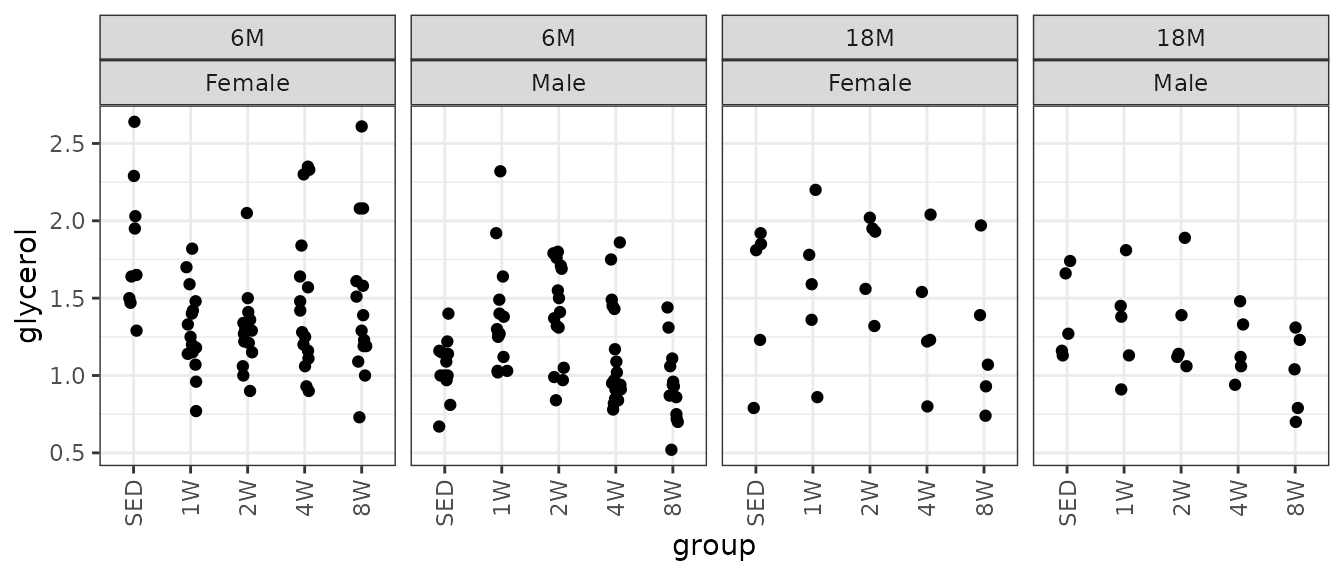
We will check the mean-variance relationship.
mv <- ANALYTES %>%
  group_by(sex, group, age) %>%
  summarise(mn = mean(glycerol, na.rm = TRUE),
            vr = var(glycerol, na.rm = TRUE))

fit.mv <- lm(log(vr) ~ log(mn), data = mv)
coef(fit.mv)
#> (Intercept)     log(mn)
#>   -2.741606    2.079242
plot(log(vr) ~ log(mn), data = mv, las = 1, pch = 19,
     xlab = "log(group means)", ylab = "log(group variances)")
abline(coef(fit.mv), lwd = 2)
The slope near 2 suggest a gamma GLM may be appropriate.
fit.glycerol <- glm(glycerol ~ age * sex * group,
                    family = Gamma("log"),
                    data = ANALYTES)
plot_lm(fit.glycerol)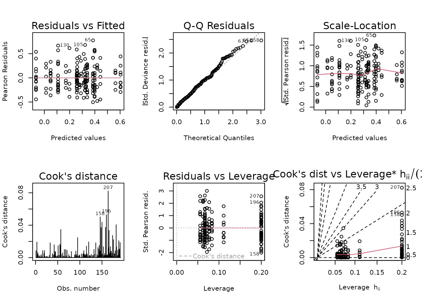
The diagnostic plots look fine. We will try to simplify the model.
anova(fit.glycerol, test = "F")
#> Analysis of Deviance Table
#>
#> Model: Gamma, link: log
#>
#> Response: glycerol
#>
#> Terms added sequentially (first to last)
#>
#>
#>               Df Deviance Resid. Df Resid. Dev       F    Pr(>F)
#> NULL                            191     17.198
#> age            1  0.06190       190     17.136  0.8627 0.3542721
#> sex            1  1.74132       189     15.395 24.2717 1.954e-06 ***
#> group          4  0.86834       185     14.526  3.0259 0.0191942 *
#> age:sex        1  0.01313       184     14.513  0.1830 0.6693131
#> age:group      4  0.14560       180     14.368  0.5074 0.7303703
#> sex:group      4  1.45233       176     12.915  5.0609 0.0007024 ***
#> age:sex:group  4  0.85400       172     12.061  2.9759 0.0207976 *
#> ---
#> Signif. codes:  0 '***' 0.001 '**' 0.01 '*' 0.05 '.' 0.1 ' ' 1
The 3-way interaction is significant, so we will not remove any terms.
summary(fit.glycerol)
#>
#> Call:
#> glm(formula = glycerol ~ age * sex * group, family = Gamma("log"),
#>     data = ANALYTES)
#>
#> Coefficients:
#>                         Estimate Std. Error t value Pr(>|t|)
#> (Intercept)             0.603709   0.089283   6.762 2.04e-10 ***
#> age18M                 -0.184998   0.149398  -1.238  0.21730
#> sexMale                -0.554125   0.118110  -4.692 5.51e-06 ***
#> group1W                -0.343398   0.112935  -3.041  0.00273 **
#> group2W                -0.347001   0.112935  -3.073  0.00247 **
#> group4W                -0.205772   0.111603  -1.844  0.06694 .
#> group8W                -0.218446   0.114437  -1.909  0.05794 .
#> age18M:sexMale          0.466156   0.206511   2.257  0.02525 *
#> age18M:group1W          0.368090   0.203596   1.808  0.07236 .
#> age18M:group2W          0.491330   0.203596   2.413  0.01686 *
#> age18M:group4W          0.098948   0.202860   0.488  0.62634
#> age18M:group8W         -0.001413   0.204433  -0.007  0.99449
#> sexMale:group1W         0.616381   0.153348   4.019 8.71e-05 ***
#> sexMale:group2W         0.636743   0.153348   4.152 5.17e-05 ***
#> sexMale:group4W         0.265043   0.149732   1.770  0.07848 .
#> sexMale:group8W         0.102887   0.156822   0.656  0.51265
#> age18M:sexMale:group1W -0.682135   0.284446  -2.398  0.01755 *
#> age18M:sexMale:group2W -0.834181   0.284446  -2.933  0.00382 **
#> age18M:sexMale:group4W -0.318374   0.282513  -1.127  0.26134
#> age18M:sexMale:group8W -0.199866   0.286334  -0.698  0.48611
#> ---
#> Signif. codes:  0 '***' 0.001 '**' 0.01 '*' 0.05 '.' 0.1 ' ' 1
#>
#> (Dispersion parameter for Gamma family taken to be 0.07174256)
#>
#>     Null deviance: 17.198  on 191  degrees of freedom
#> Residual deviance: 12.061  on 172  degrees of freedom
#>   (90 observations deleted due to missingness)
#> AIC: 148.8
#>
#> Number of Fisher Scoring iterations: 4
Insulin
Insulin (pM). It does not matter which units we use for insulin. It does not affect the model fit or the ratios when we set up the comparisons later.
# Plot points
ggplot(ANALYTES, aes(x = group, y = insulin_pm)) +
  geom_point(position = position_jitter(width = 0.1, height = 0),
             na.rm = TRUE) +
  facet_wrap(~ age + sex, nrow = 1) +
  theme(axis.text.x = element_text(angle = 90, hjust = 1, vjust = 0.5))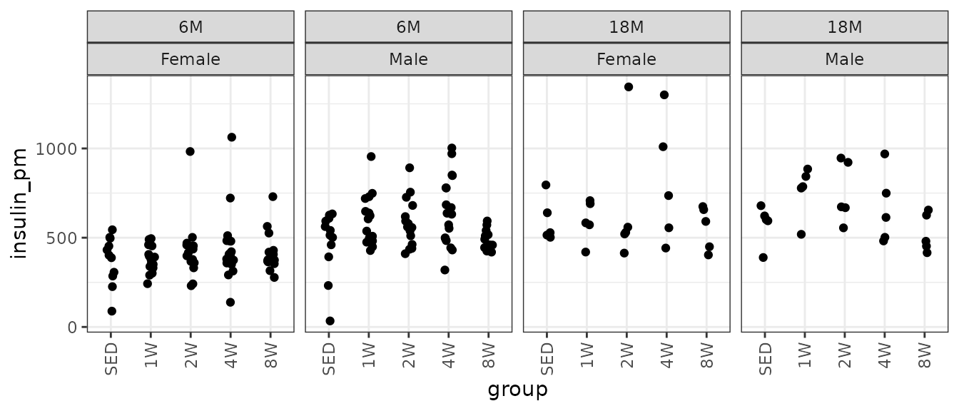
There are extremely large values in the 2W Female group at both ages, though they are comparable to values from their corresponding 4W groups. We will check the mean-variance relationship.
mv <- ANALYTES %>%
  group_by(sex, group, age) %>%
  summarise(mn = mean(insulin_pm, na.rm = TRUE),
            vr = var(insulin_pm, na.rm = TRUE))

fit.mv <- lm(log(vr) ~ log(mn), data = mv)
coef(fit.mv)
#> (Intercept)     log(mn)
#>   -2.263771    1.937433
plot(log(vr) ~ log(mn), data = mv, las = 1, pch = 19,
     xlab = "log(group means)", ylab = "log(group variances)")
abline(coef(fit.mv), lwd = 2)
The slope is close to 2, so a gamma GLM may be appropriate.
fit.ins <- glm(insulin_pm ~ age * sex * group,
               family = Gamma("log"),
               data = ANALYTES)
plot_lm(fit.ins)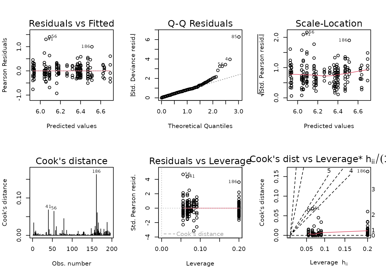
The gamma distribution is sensitive to large outlying values, which we observed when plotting insulin. We will try a log-link Gaussian with reciprocal group variances as weights.
wt.ins <- ANALYTES %>%
  group_by(age, sex, group) %>%
  mutate(1 / var(insulin_pm, na.rm = TRUE)) %>%
  pull(-1)

fit.ins <- update(fit.ins,
                  family = gaussian("log"),
                  weights = wt.ins)
plot_lm(fit.ins)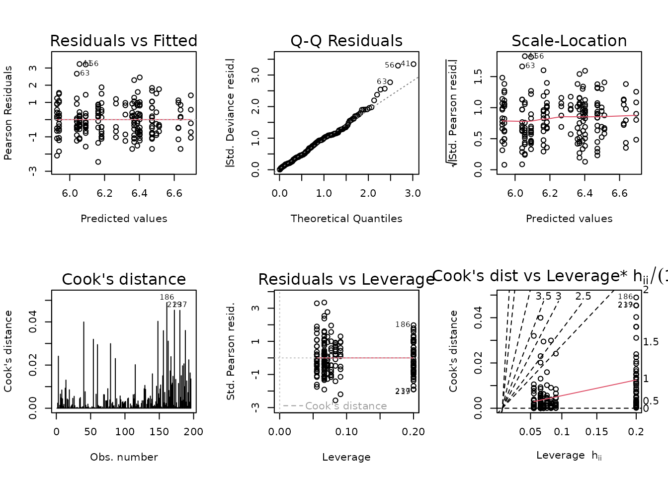
The diagnostic plots look fine now. We will try to simplify the model.
anova(fit.ins, test = "F")
#> Analysis of Deviance Table
#>
#> Model: gaussian, link: log
#>
#> Response: insulin_pm
#>
#> Terms added sequentially (first to last)
#>
#>
#>               Df Deviance Resid. Df Resid. Dev       F    Pr(>F)
#> NULL                            195     305.98
#> age            1   43.004       194     262.97 43.0039 5.860e-10 ***
#> sex            1   38.458       193     224.51 38.4581 3.874e-09 ***
#> group          4   21.242       189     203.27  5.3105 0.0004628 ***
#> age:sex        1   12.650       188     190.62 12.6501 0.0004826 ***
#> age:group      4    1.949       184     188.67  0.4873 0.7450724
#> sex:group      4   11.067       180     177.61  2.7667 0.0289877 *
#> age:sex:group  4    1.607       176     176.00  0.4019 0.8071332
#> ---
#> Signif. codes:  0 '***' 0.001 '**' 0.01 '*' 0.05 '.' 0.1 ' ' 1
We will remove the group:age and 3-way interactions.
fit.ins.1 <- update(fit.ins,
                    formula = . ~ sex * (age + group))
fit.ins.2 <- update(fit.ins,
                    formula = . ~ (age + sex + group) ^ 2)
anova(fit.ins.1, fit.ins.2, fit.ins, test = "F")
#> Analysis of Deviance Table
#>
#> Model 1: insulin_pm ~ sex + age + group + sex:age + sex:group
#> Model 2: insulin_pm ~ age + sex + group + age:sex + age:group + sex:group
#> Model 3: insulin_pm ~ age * sex * group
#>   Resid. Df Resid. Dev Df Deviance      F Pr(>F)
#> 1       184     180.85
#> 2       180     177.61  4   3.2462 0.8116 0.5193
#> 3       176     176.00  4   1.6075 0.4019 0.8071
No significant differences between the models, so we will use the simplest one.
fit.ins <- fit.ins.1
plot_lm(fit.ins)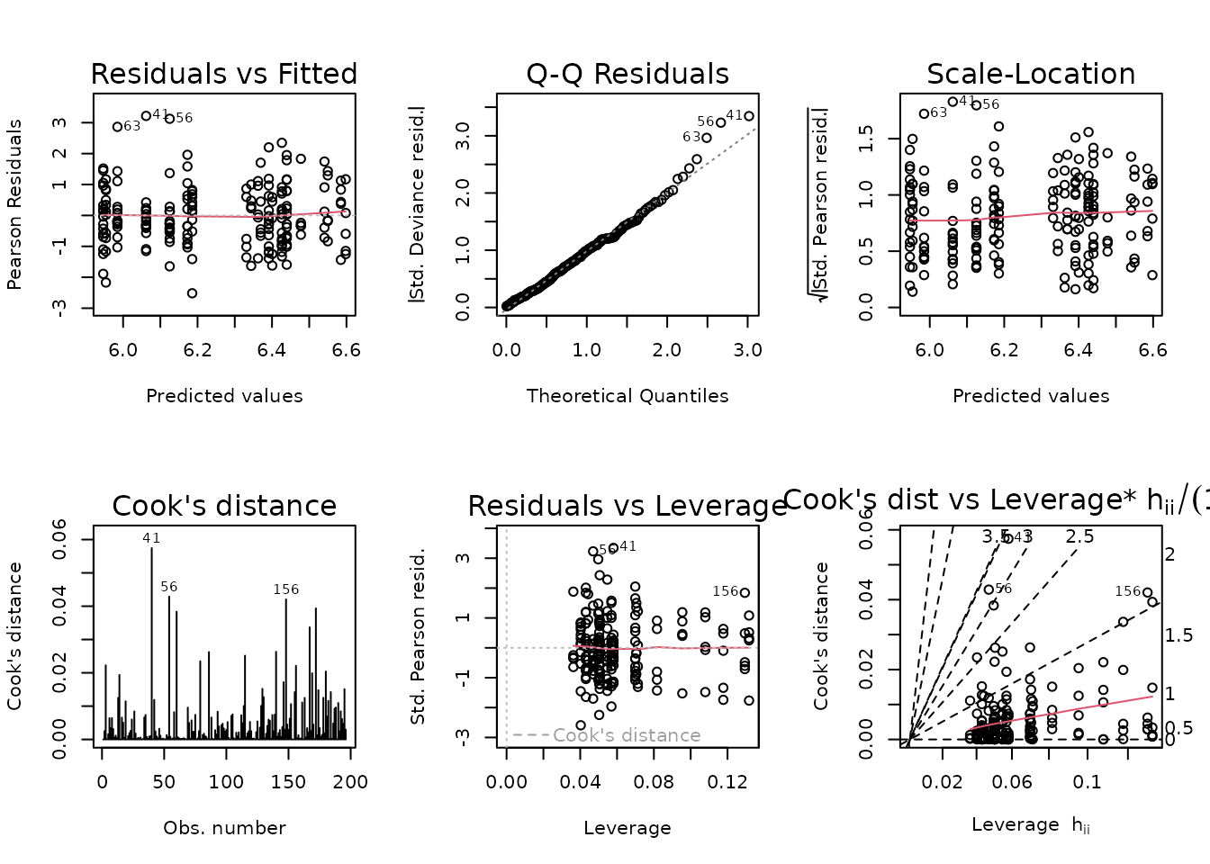
summary(fit.ins)
#>
#> Call:
#> glm(formula = insulin_pm ~ sex + age + group + sex:age + sex:group,
#>     family = gaussian("log"), data = ANALYTES, weights = wt.ins)
#>
#> Coefficients:
#>                  Estimate Std. Error t value Pr(>|t|)
#> (Intercept)      5.953791   0.078922  75.439  < 2e-16 ***
#> sexMale          0.231786   0.107888   2.148  0.03299 *
#> age18M           0.415816   0.063548   6.543 5.79e-10 ***
#> group1W         -0.007132   0.085140  -0.084  0.93333
#> group2W          0.107991   0.121619   0.888  0.37573
#> group4W          0.171370   0.117420   1.459  0.14614
#> group8W          0.030930   0.092174   0.336  0.73758
#> sexMale:age18M  -0.257350   0.081706  -3.150  0.00191 **
#> sexMale:group1W  0.248068   0.119721   2.072  0.03965 *
#> sexMale:group2W  0.097820   0.149081   0.656  0.51254
#> sexMale:group4W  0.082580   0.149639   0.552  0.58171
#> sexMale:group8W -0.043708   0.120389  -0.363  0.71698
#> ---
#> Signif. codes:  0 '***' 0.001 '**' 0.01 '*' 0.05 '.' 0.1 ' ' 1
#>
#> (Dispersion parameter for gaussian family taken to be 0.9829014)
#>
#>     Null deviance: 305.98  on 195  degrees of freedom
#> Residual deviance: 180.85  on 184  degrees of freedom
#>   (86 observations deleted due to missingness)
#> AIC: 2506.2
#>
#> Number of Fisher Scoring iterations: 5
Ketones
Ketones (\(\mu\)mol/L).
# Plot points
ggplot(ANALYTES, aes(x = group, y = ketones)) +
  geom_point(position = position_jitter(width = 0.1, height = 0),
             na.rm = TRUE) +
  facet_wrap(~ age + sex, nrow = 1) +
  theme(axis.text.x = element_text(angle = 90, hjust = 1, vjust = 0.5))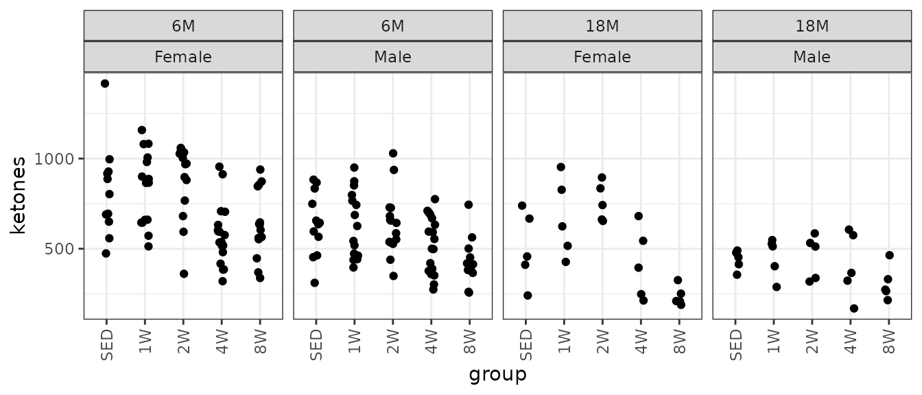
We will check the mean-variance relationship.
mv <- ANALYTES %>%
  group_by(sex, group, age) %>%
  summarise(mn = mean(ketones, na.rm = TRUE),
            vr = var(ketones, na.rm = TRUE))

fit.mv <- lm(log(vr) ~ log(mn), data = mv)
coef(fit.mv)
#> (Intercept)     log(mn)
#>  -0.8087957   1.7185456
plot(log(vr) ~ log(mn), data = mv, las = 1, pch = 19,
     xlab = "log(group means)", ylab = "log(group variances)")
abline(coef(fit.mv), lwd = 2)
The slope of the line is close to 2, suggesting a gamma GLM may be appropriate.
fit.ket <- glm(ketones ~ sex * group * age,
               family = Gamma("log"),
               data = ANALYTES)
plot_lm(fit.ket)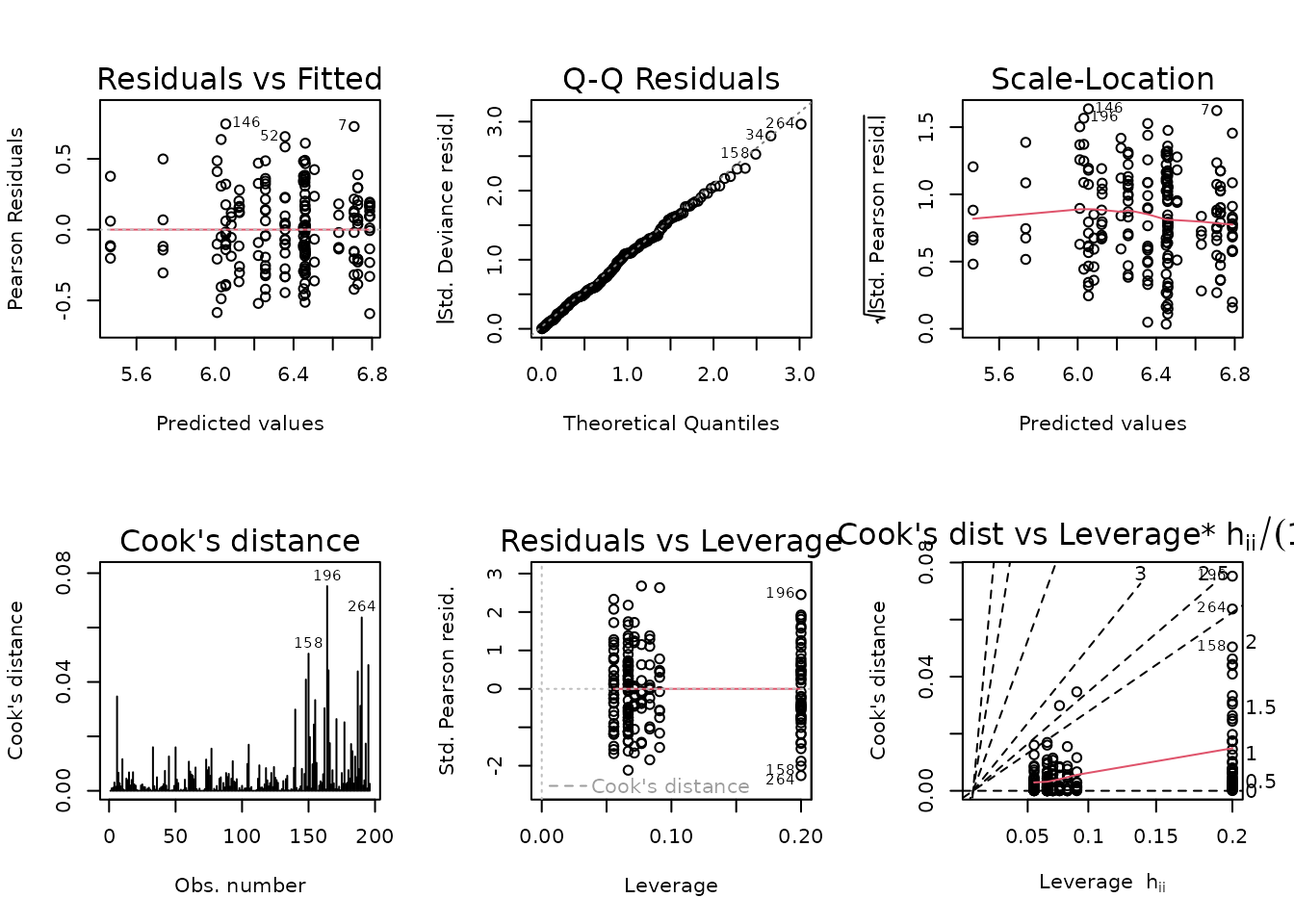
The diagnostic plots look fine. We will try to simplify the model.
anova(fit.ket, test = "F")
#> Analysis of Deviance Table
#>
#> Model: Gamma, link: log
#>
#> Response: ketones
#>
#> Terms added sequentially (first to last)
#>
#>
#>               Df Deviance Resid. Df Resid. Dev       F    Pr(>F)
#> NULL                            195     31.057
#> sex            1   3.0984       194     27.958 36.8486 7.644e-09 ***
#> group          4   5.6087       190     22.349 16.6755 1.318e-11 ***
#> age            1   4.5876       189     17.762 54.5590 5.811e-12 ***
#> sex:group      4   0.5164       185     17.245  1.5353   0.19394
#> sex:age        1   0.0731       184     17.172  0.8697   0.35232
#> group:age      4   0.7610       180     16.411  2.2626   0.06429 .
#> sex:group:age  4   0.8083       176     15.603  2.4033   0.05157 .
#> ---
#> Signif. codes:  0 '***' 0.001 '**' 0.01 '*' 0.05 '.' 0.1 ' ' 1
The 3-way interaction is marginally significant, so we will not simplify the model.
summary(fit.ket)
#>
#> Call:
#> glm(formula = ketones ~ sex * group * age, family = Gamma("log"),
#>     data = ANALYTES)
#>
#> Coefficients:
#>                        Estimate Std. Error t value Pr(>|t|)
#> (Intercept)             6.70853    0.08743  76.729  < 2e-16 ***
#> sexMale                -0.24993    0.12104  -2.065  0.04041 *
#> group1W                 0.01858    0.11511   0.161  0.87192
#> group2W                 0.07947    0.11511   0.690  0.49087
#> group4W                -0.35175    0.11098  -3.170  0.00180 **
#> group8W                -0.25772    0.11683  -2.206  0.02869 *
#> age18M                 -0.48794    0.15640  -3.120  0.00212 **
#> sexMale:group1W        -0.01905    0.16082  -0.118  0.90582
#> sexMale:group2W        -0.07806    0.16082  -0.485  0.62801
#> sexMale:group4W         0.15007    0.15490   0.969  0.33397
#> sexMale:group8W        -0.14608    0.16470  -0.887  0.37631
#> sexMale:age18M          0.11201    0.21974   0.510  0.61086
#> group1W:age18M          0.26721    0.21653   1.234  0.21883
#> group2W:age18M          0.33010    0.21653   1.525  0.12918
#> group4W:age18M          0.16232    0.21436   0.757  0.44992
#> group8W:age18M         -0.49566    0.21745  -2.279  0.02384 *
#> sexMale:group1W:age18M -0.22736    0.30517  -0.745  0.45726
#> sexMale:group2W:age18M -0.28950    0.30517  -0.949  0.34411
#> sexMale:group4W:age18M -0.03254    0.30210  -0.108  0.91434
#> sexMale:group8W:age18M  0.55206    0.30724   1.797  0.07407 .
#> ---
#> Signif. codes:  0 '***' 0.001 '**' 0.01 '*' 0.05 '.' 0.1 ' ' 1
#>
#> (Dispersion parameter for Gamma family taken to be 0.08408593)
#>
#>     Null deviance: 31.057  on 195  degrees of freedom
#> Residual deviance: 15.603  on 176  degrees of freedom
#>   (86 observations deleted due to missingness)
#> AIC: 2586.3
#>
#> Number of Fisher Scoring iterations: 4
Lactate
Lactate (mmol/L).
# Plot points
ggplot(ANALYTES, aes(x = group, y = lactate)) +
  geom_point(position = position_jitter(width = 0.1, height = 0),
             na.rm = TRUE) +
  facet_wrap(~ age + sex, nrow = 1) +
  theme(axis.text.x = element_text(angle = 90, hjust = 1, vjust = 0.5))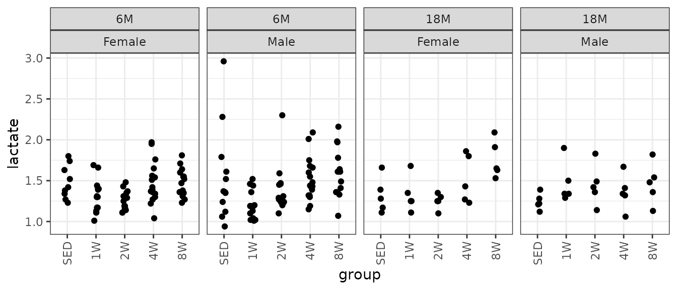
The large value in the 6M SED Male group may be an outlier. There is also a large value in the 2W group. We will check the mean-variance relationship.
mv <- ANALYTES %>%
  group_by(sex, group, age) %>%
  summarise(mn = mean(lactate, na.rm = TRUE),
            vr = var(lactate, na.rm = TRUE))

fit.mv <- lm(log(vr) ~ log(mn), data = mv)
coef(fit.mv)
#> (Intercept)     log(mn)
#>   -5.022331    5.637233
plot(log(vr) ~ log(mn), data = mv, las = 1, pch = 19,
     xlab = "log(group means)", ylab = "log(group variances)")
abline(coef(fit.mv), lwd = 2)
The slope of the line is close to 6! We will try a log-link Gaussian GLM with inverse group variance weights.
wt.lact <- ANALYTES %>%
  group_by(age, sex, group) %>%
  mutate(1 / var(lactate, na.rm = TRUE)) %>%
  pull(-1)

fit.lact <- glm(lactate ~ age * sex * group,
                family = gaussian("log"),
                weights = wt.lact,
                data = ANALYTES)
plot_lm(fit.lact)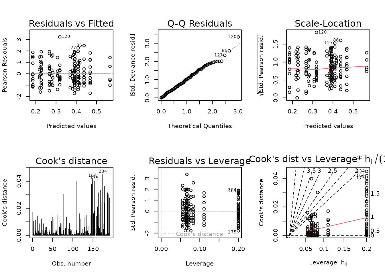
We will try to simplify the model to improve the diagnostics.
anova(fit.lact, test = "F")
#> Analysis of Deviance Table
#>
#> Model: gaussian, link: log
#>
#> Response: lactate
#>
#> Terms added sequentially (first to last)
#>
#>
#>               Df Deviance Resid. Df Resid. Dev       F    Pr(>F)
#> NULL                            191     258.27
#> age            1    0.768       190     257.51  0.7685  0.381914
#> sex            1    0.000       189     257.51  0.0000  0.996278
#> group          4   55.274       185     202.23 13.8183 8.571e-10 ***
#> age:sex        1    1.790       184     200.44  1.7897  0.182724
#> age:group      4   13.915       180     186.53  3.4787  0.009243 **
#> sex:group      4    5.703       176     180.82  1.4258  0.227441
#> age:sex:group  4    8.824       172     172.00  2.2061  0.070325 .
#> ---
#> Signif. codes:  0 '***' 0.001 '**' 0.01 '*' 0.05 '.' 0.1 ' ' 1
fit.lact.1 <- update(fit.lact, formula = . ~ age * group + sex)
anova(fit.lact.1, fit.lact, test = "F")
#> Analysis of Deviance Table
#>
#> Model 1: lactate ~ age + group + sex + age:group
#> Model 2: lactate ~ age * sex * group
#>   Resid. Df Resid. Dev Df Deviance      F  Pr(>F)
#> 1       181     187.09
#> 2       172     172.00  9   15.091 1.6768 0.09786 .
#> ---
#> Signif. codes:  0 '***' 0.001 '**' 0.01 '*' 0.05 '.' 0.1 ' ' 1
There is no significant difference between the models, so we will use the simpler one.
fit.lact <- fit.lact.1
plot_lm(fit.lact)
The diagnostic plots look better.
summary(fit.lact)
#>
#> Call:
#> glm(formula = lactate ~ age + group + sex + age:group, family = gaussian("log"),
#>     data = ANALYTES, weights = wt.lact)
#>
#> Coefficients:
#>                 Estimate Std. Error t value Pr(>|t|)
#> (Intercept)     0.398546   0.043061   9.255  < 2e-16 ***
#> age18M         -0.175327   0.056484  -3.104 0.002216 **
#> group1W        -0.182192   0.051803  -3.517 0.000552 ***
#> group2W        -0.158544   0.048356  -3.279 0.001251 **
#> group4W        -0.001806   0.053137  -0.034 0.972925
#> group8W         0.010868   0.050979   0.213 0.831427
#> sexMale         0.007122   0.024449   0.291 0.771154
#> age18M:group1W  0.285175   0.083121   3.431 0.000745 ***
#> age18M:group2W  0.176902   0.068426   2.585 0.010516 *
#> age18M:group4W  0.121508   0.084703   1.435 0.153149
#> age18M:group8W  0.249203   0.077829   3.202 0.001613 **
#> ---
#> Signif. codes:  0 '***' 0.001 '**' 0.01 '*' 0.05 '.' 0.1 ' ' 1
#>
#> (Dispersion parameter for gaussian family taken to be 1.033653)
#>
#>     Null deviance: 258.28  on 191  degrees of freedom
#> Residual deviance: 187.09  on 181  degrees of freedom
#>   (90 observations deleted due to missingness)
#> AIC: -15.338
#>
#> Number of Fisher Scoring iterations: 5
Leptin
Leptin (pg/mL).
# Plot points
ggplot(ANALYTES, aes(x = group, y = leptin)) +
  geom_point(position = position_jitter(width = 0.1, height = 0),
             na.rm = TRUE) +
  facet_wrap(~ age + sex, nrow = 1) +
  theme(axis.text.x = element_text(angle = 90, hjust = 1, vjust = 0.5))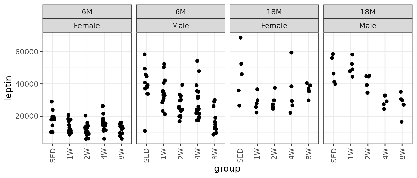
There are a few large outlying values. We will check the mean-variance relationship.
mv <- ANALYTES %>%
  group_by(sex, group, age) %>%
  summarise(mn = mean(leptin, na.rm = TRUE),
            vr = var(leptin, na.rm = TRUE))

fit.mv <- lm(log(vr) ~ log(mn), data = mv)
coef(fit.mv)
#> (Intercept)     log(mn)
#>    6.275343    1.098834
plot(log(vr) ~ log(mn), data = mv, las = 1, pch = 19,
     xlab = "log(group means)", ylab = "log(group variances)")
abline(coef(fit.mv), lwd = 2)
The slope is close to 1, so we will use a quasi-Poisson distribution, since we are not dealing with count data.
fit.lep <- glm(leptin ~ age * sex * group,
               family = quasipoisson("log"),
               data = ANALYTES)
plot_lm(fit.lep)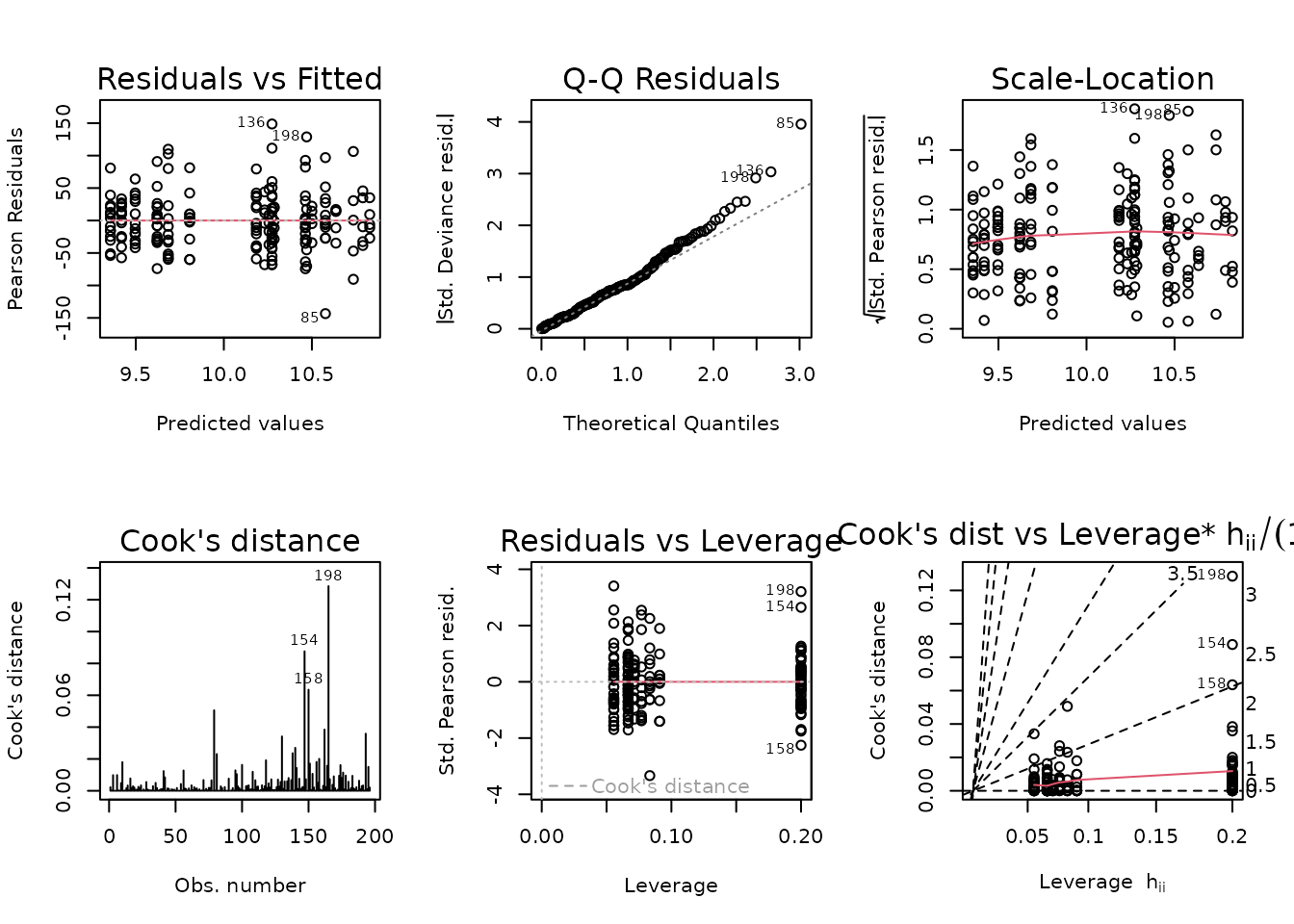
Observations are deviating from the right tail of the QQ-plot. We will fit a log-link Gaussian GLM with inverse group variance weights.
wt.lep <- ANALYTES %>%
  group_by(age, sex, group) %>%
  mutate(1 / var(leptin, na.rm = TRUE)) %>%
  pull(-1)

fit.lep <- update(fit.lep,
                  family = gaussian("log"),
                  weights = wt.lep)
plot_lm(fit.lep)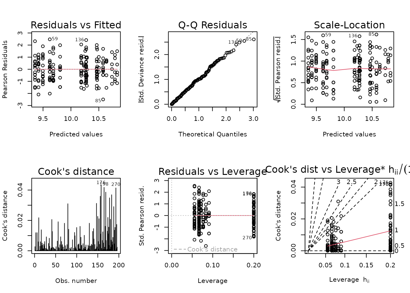
The diagnostic plots look fine. We will try to simplify the model.
anova(fit.lep, test = "F")
#> Analysis of Deviance Table
#>
#> Model: gaussian, link: log
#>
#> Response: leptin
#>
#> Terms added sequentially (first to last)
#>
#>
#>               Df Deviance Resid. Df Resid. Dev        F    Pr(>F)
#> NULL                            195    1014.00
#> age            1   495.90       194     518.10 495.9023 < 2.2e-16 ***
#> sex            1   111.23       193     406.86 111.2346 < 2.2e-16 ***
#> group          4    74.77       189     332.09  18.6936 8.005e-13 ***
#> age:sex        1    62.23       188     269.86  62.2254 3.116e-13 ***
#> age:group      4    32.67       184     237.19   8.1674 4.595e-06 ***
#> sex:group      4    57.74       180     179.45  14.4352 3.260e-10 ***
#> age:sex:group  4     3.45       176     176.00   0.8630    0.4874
#> ---
#> Signif. codes:  0 '***' 0.001 '**' 0.01 '*' 0.05 '.' 0.1 ' ' 1
We will remove the 3-way interaction.
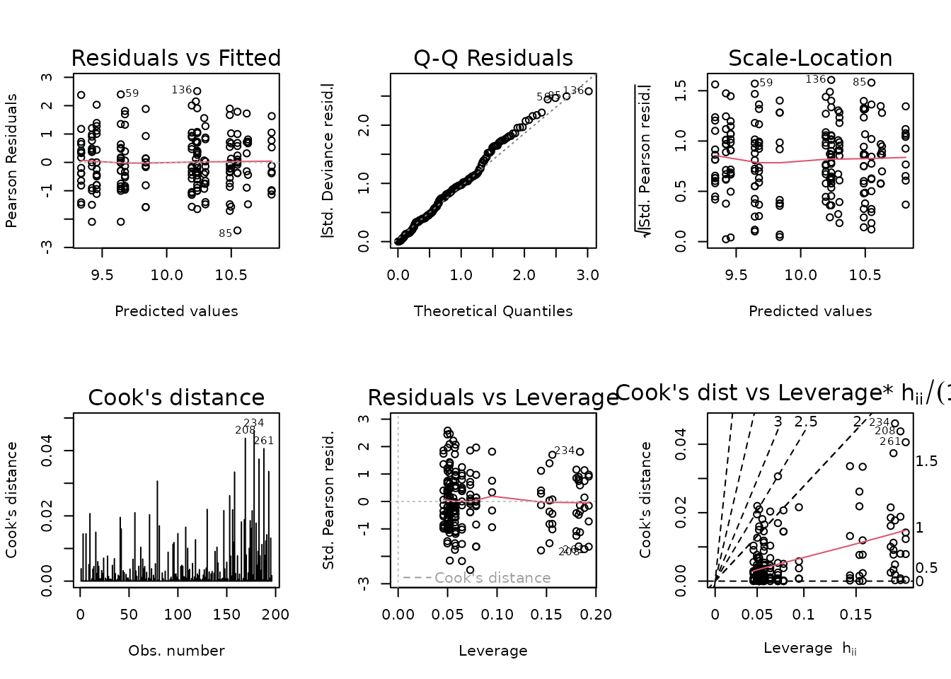
summary(fit.lep)
#>
#> Call:
#> glm(formula = leptin ~ age + sex + group + age:sex + age:group +
#>     sex:group, family = gaussian("log"), data = ANALYTES, weights = wt.lep)
#>
#> Coefficients:
#>                 Estimate Std. Error t value Pr(>|t|)
#> (Intercept)      9.83738    0.08236 119.447  < 2e-16 ***
#> age18M           0.78252    0.11513   6.797 1.52e-10 ***
#> sexMale          0.71056    0.10623   6.689 2.74e-10 ***
#> group1W         -0.38005    0.10468  -3.631 0.000368 ***
#> group2W         -0.50031    0.10730  -4.663 6.07e-06 ***
#> group4W         -0.19300    0.10538  -1.831 0.068697 .
#> group8W         -0.41667    0.10238  -4.070 7.03e-05 ***
#> age18M:sexMale  -0.51809    0.07817  -6.628 3.82e-10 ***
#> age18M:group1W   0.06037    0.11838   0.510 0.610696
#> age18M:group2W   0.17099    0.11886   1.439 0.151993
#> age18M:group4W  -0.20094    0.13811  -1.455 0.147441
#> age18M:group8W   0.29560    0.13201   2.239 0.026371 *
#> sexMale:group1W  0.32090    0.12564   2.554 0.011475 *
#> sexMale:group2W  0.14665    0.12670   1.157 0.248641
#> sexMale:group4W -0.11858    0.14571  -0.814 0.416805
#> sexMale:group8W -0.45445    0.14257  -3.187 0.001693 **
#> ---
#> Signif. codes:  0 '***' 0.001 '**' 0.01 '*' 0.05 '.' 0.1 ' ' 1
#>
#> (Dispersion parameter for gaussian family taken to be 0.9969575)
#>
#>     Null deviance: 1014.00  on 195  degrees of freedom
#> Residual deviance:  179.45  on 180  degrees of freedom
#>   (86 observations deleted due to missingness)
#> AIC: 3988
#>
#> Number of Fisher Scoring iterations: 5
NEFA
NEFA (mmol/L).
# Plot points
ggplot(ANALYTES, aes(x = group, y = nefa)) +
  geom_point(position = position_jitter(width = 0.1, height = 0),
             na.rm = TRUE) +
  facet_wrap(~ age + sex, nrow = 1) +
  theme(axis.text.x = element_text(angle = 90, hjust = 1, vjust = 0.5))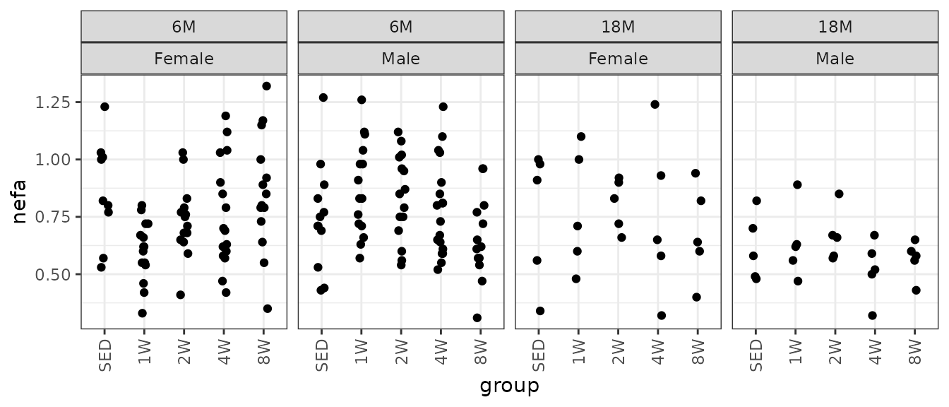
We will check the mean-variance relationship.
mv <- ANALYTES %>%
  group_by(sex, group, age) %>%
  summarise(mn = mean(nefa, na.rm = TRUE),
            vr = var(nefa, na.rm = TRUE))

fit.mv <- lm(log(vr) ~ log(mn), data = mv)
coef(fit.mv)
#> (Intercept)     log(mn)
#>   -2.400661    3.016098
plot(log(vr) ~ log(mn), data = mv, las = 1, pch = 19,
     xlab = "log(group means)", ylab = "log(group variances)")
abline(coef(fit.mv), lwd = 2)
The slope of the line is close to 3, suggesting the group variance is proportional to the cube of the group mean. This corresponds to an inverse Gaussian distribution.
fit.nefa <- glm(nefa ~ sex * group * age,
                family = inverse.gaussian("log"),
                data = ANALYTES)
plot_lm(fit.nefa)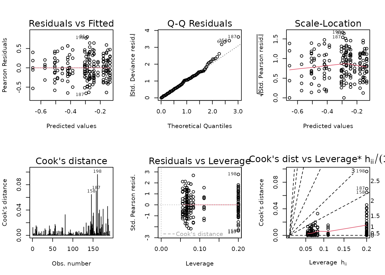
The diagnostic plots look fine. We will try to simplify the model.
anova(fit.nefa, test = "F")
#> Analysis of Deviance Table
#>
#> Model: inverse.gaussian, link: log
#>
#> Response: nefa
#>
#> Terms added sequentially (first to last)
#>
#>
#>               Df Deviance Resid. Df Resid. Dev       F   Pr(>F)
#> NULL                            191     24.007
#> sex            1  0.02874       190     23.978  0.2962 0.586957
#> group          4  0.17576       186     23.803  0.4528 0.770222
#> age            1  0.92850       185     22.874  9.5691 0.002310 **
#> sex:group      4  1.54674       181     21.327  3.9852 0.004059 **
#> sex:age        1  1.01386       180     20.314 10.4489 0.001471 **
#> group:age      4  0.27725       176     20.036  0.7143 0.583187
#> sex:group:age  4  0.70055       172     19.336  1.8050 0.130020
#> ---
#> Signif. codes:  0 '***' 0.001 '**' 0.01 '*' 0.05 '.' 0.1 ' ' 1
We will remove the group:age and 3-way interaction and
compare the models.
fit.nefa.1 <- update(fit.nefa, formula = . ~ sex * (group + age))
anova(fit.nefa.1, fit.nefa, test = "F")
#> Analysis of Deviance Table
#>
#> Model 1: nefa ~ sex + group + age + sex:group + sex:age
#> Model 2: nefa ~ sex * group * age
#>   Resid. Df Resid. Dev Df Deviance      F Pr(>F)
#> 1       180     20.314
#> 2       172     19.336  8   0.9778 1.2597 0.2677
There is no significant difference between the models, so we will use the simpler one.
fit.nefa <- fit.nefa.1
plot_lm(fit.nefa)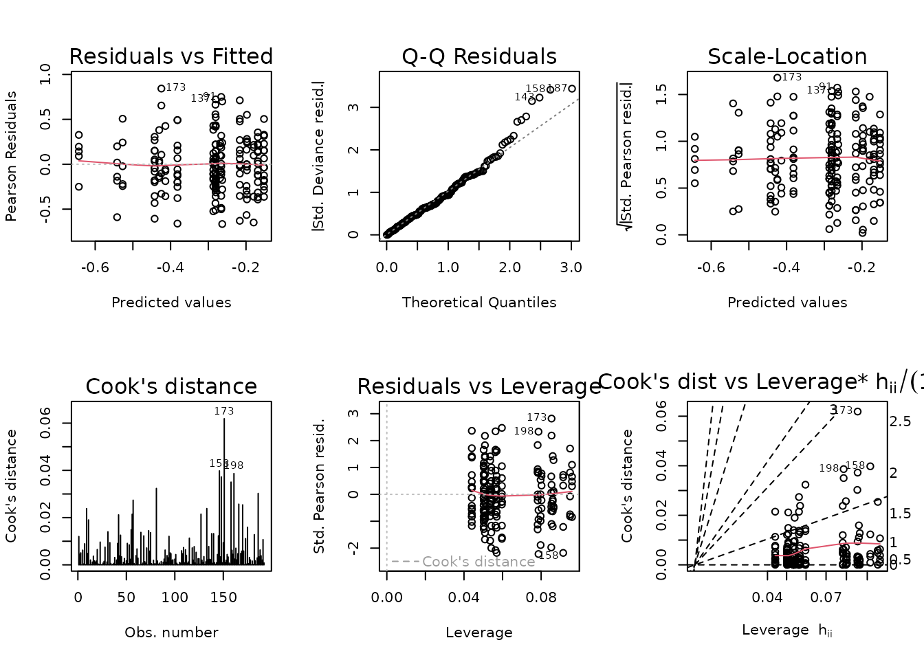
summary(fit.nefa)
#>
#> Call:
#> glm(formula = nefa ~ sex + group + age + sex:group + sex:age,
#>     family = inverse.gaussian("log"), data = ANALYTES)
#>
#> Coefficients:
#>                 Estimate Std. Error t value Pr(>|t|)
#> (Intercept)     -0.19762    0.07918  -2.496  0.01346 *
#> sexMale         -0.06804    0.10362  -0.657  0.51222
#> group1W         -0.24475    0.09466  -2.586  0.01051 *
#> group2W         -0.08907    0.09742  -0.914  0.36183
#> group4W         -0.08334    0.09668  -0.862  0.38980
#> group8W         -0.01884    0.09979  -0.189  0.85045
#> age18M           0.01790    0.06373   0.281  0.77912
#> sexMale:group1W  0.35813    0.13008   2.753  0.00651 **
#> sexMale:group2W  0.18606    0.13186   1.411  0.15996
#> sexMale:group4W  0.06869    0.12819   0.536  0.59274
#> sexMale:group8W -0.09727    0.13202  -0.737  0.46220
#> sexMale:age18M  -0.27944    0.08633  -3.237  0.00144 **
#> ---
#> Signif. codes:  0 '***' 0.001 '**' 0.01 '*' 0.05 '.' 0.1 ' ' 1
#>
#> (Dispersion parameter for inverse.gaussian family taken to be 0.09767937)
#>
#>     Null deviance: 24.007  on 191  degrees of freedom
#> Residual deviance: 20.314  on 180  degrees of freedom
#>   (90 observations deleted due to missingness)
#> AIC: -54.315
#>
#> Number of Fisher Scoring iterations: 6
Hypothesis Testing
We will compare the means of each trained timepoint to those of their sex-matched sedentary controls within each age group using the Dunnett test. This is a multiple comparison procedure to compare each of several treatment groups (1W, 2W, 4W, 8W) against a single control group (SED). The assumptions of this test are that the observations in each group are independent and identically distributed with equal variances. We have already checked that these assumptions were satisfied with the regression diagnostic plots.
If the response had been transformed, tests and interpretation will be done on the transformed scale to avoid introducing bias when back-transforming.
# Create emm_list objects
model_list <- list("Corticosterone" = fit.cort,
                   "Glucagon" = fit.glucagon,
                   "Glucose" = fit.glucose,
                   "Glycerol" = fit.glycerol,
                   "Insulin" = fit.ins,
                   "Ketones" = fit.ket,
                   "Lactate" = fit.lact,
                   "Leptin" = fit.lep,
                   "NEFA" = fit.nefa)

# List of emmGrid objects
ANALYTES_EMM <- map(model_list, function(mod_i) {
  terms_i <- attr(terms(mod_i), which = "term.labels")
  by <- intersect(c("age", "sex"), terms_i)

  if (length(by) == 0) {
    by <- NULL
  }

  emmeans(mod_i, specs = "group", by = by,
          type = "response", infer = TRUE)
})
# Extract model info
model_df <- model_list %>%
  map_chr(.f = ~ paste(deparse(.x[["call"]]), collapse = "")) %>%
  enframe(name = "response", value = "model") %>%
  mutate(model = gsub("(?<=[\\s])\\s*|^\\s+|\\s+$", "", model, perl = TRUE),
         model_type = sub("^([^\\(]+).*", "\\1", model),
         family = sub(".*family = ([^\\)]+\\)),.*", "\\1", model),
         formula = sub(".*formula = ([^,]+),.*", "\\1", model),
         family = ifelse(model_type == "lm", "gaussian", family),
         # if weights were used, they were inverse group variances
         weights = ifelse(grepl("weights = ", model),
                          "inverse group variances", NA)) %>%
  select(-model)
# Results
ANALYTES_STATS <- ANALYTES_EMM %>%
  map(function(emm_i) {
    # "trt.vs.ctrl" and "dunnett" are interchangeable
    contrast(emm_i, method = "trt.vs.ctrl") %>%
      summary(infer = TRUE) %>%
      as.data.frame() %>%
      # Rename asymptotic confidence interval columns (quasi-distributions) to
      # simplify output
      rename(any_of(c(lower.CL = "asymp.LCL",
                      upper.CL = "asymp.UCL")))
  }) %>%
  enframe(name = "response") %>%
  unnest(value) %>%
  # In cases where either age or sex was not included as a predictor,
  # we will duplicate those rows and fill in those column entries.
  mutate(age = ifelse(is.na(age), "6M, 18M", as.character(age)),
         sex = ifelse(is.na(sex), "Female, Male", as.character(sex))) %>%
  separate_longer_delim(cols = c(age, sex), delim = ", ") %>%
  pivot_longer(cols = ratio,
               names_to = "estimate_type",
               values_to = "estimate",
               values_drop_na = TRUE) %>%
  pivot_longer(cols = contains(".ratio"),
               names_to = "statistic_type",
               values_to = "statistic",
               values_drop_na = TRUE) %>%
  # p-values are actually Dunnett p-values (already adjusted)
  dplyr::rename(p.adj = p.value) %>%
  mutate(statistic_type = sub("\\.ratio", "", statistic_type),
         age = factor(age, levels = c("6M", "18M")),
         sex = factor(sex, levels = c("Female", "Male")),
         # Calculate two-sided p-values
         p.value = 2 * pt(q = estimate, df = df, lower.tail = FALSE),
         signif = p.adj < 0.05) %>%
  left_join(model_df, by = "response") %>%
  # Reorder columns
  dplyr::select(response, age, sex, contrast, estimate_type, null, estimate, SE,
                lower.CL, upper.CL, statistic_type, statistic, df, p.value,
                p.adj, signif, model_type, family, formula, weights,
                everything()) %>%
  arrange(response, age, sex, contrast) %>%
  as.data.frame()
See ?ANALYTES_STATS for details.
print.data.frame(head(ANALYTES_STATS, 10))
#>          response age    sex contrast estimate_type null estimate        SE
#> 1  Corticosterone  6M Female 1W / SED         ratio    1 1.832279 0.2981685
#> 2  Corticosterone  6M Female 2W / SED         ratio    1 1.530332 0.2571677
#> 3  Corticosterone  6M Female 4W / SED         ratio    1 1.895274 0.2778634
#> 4  Corticosterone  6M Female 8W / SED         ratio    1 1.279948 0.2011438
#> 5  Corticosterone  6M   Male 1W / SED         ratio    1 1.832279 0.2981685
#> 6  Corticosterone  6M   Male 2W / SED         ratio    1 1.530332 0.2571677
#> 7  Corticosterone  6M   Male 4W / SED         ratio    1 1.895274 0.2778634
#> 8  Corticosterone  6M   Male 8W / SED         ratio    1 1.279948 0.2011438
#> 9  Corticosterone 18M Female 1W / SED         ratio    1 1.832279 0.2981685
#> 10 Corticosterone 18M Female 2W / SED         ratio    1 1.530332 0.2571677
#>     lower.CL upper.CL statistic_type statistic  df    p.value       p.adj
#> 1  1.2249426 2.740737              t  3.721236 189 0.06848359 0.001014465
#> 2  1.0097111 2.319392              t  2.531939 189 0.12760657 0.043071377
#> 3  1.3186265 2.724094              t  4.361023 189 0.05958248 0.000083877
#> 4  0.8675887 1.888298              t  1.570596 189 0.20213238 0.333765251
#> 5  1.2249426 2.740737              t  3.721236 189 0.06848359 0.001014465
#> 6  1.0097111 2.319392              t  2.531939 189 0.12760657 0.043071377
#> 7  1.3186265 2.724094              t  4.361023 189 0.05958248 0.000083877
#> 8  0.8675887 1.888298              t  1.570596 189 0.20213238 0.333765251
#> 9  1.2249426 2.740737              t  3.721236 189 0.06848359 0.001014465
#> 10 1.0097111 2.319392              t  2.531939 189 0.12760657 0.043071377
#>    signif model_type          family                      formula
#> 1    TRUE        glm gaussian("log") corticosterone ~ sex + group
#> 2    TRUE        glm gaussian("log") corticosterone ~ sex + group
#> 3    TRUE        glm gaussian("log") corticosterone ~ sex + group
#> 4   FALSE        glm gaussian("log") corticosterone ~ sex + group
#> 5    TRUE        glm gaussian("log") corticosterone ~ sex + group
#> 6    TRUE        glm gaussian("log") corticosterone ~ sex + group
#> 7    TRUE        glm gaussian("log") corticosterone ~ sex + group
#> 8   FALSE        glm gaussian("log") corticosterone ~ sex + group
#> 9    TRUE        glm gaussian("log") corticosterone ~ sex + group
#> 10   TRUE        glm gaussian("log") corticosterone ~ sex + group
#>                    weights
#> 1  inverse group variances
#> 2  inverse group variances
#> 3  inverse group variances
#> 4  inverse group variances
#> 5  inverse group variances
#> 6  inverse group variances
#> 7  inverse group variances
#> 8  inverse group variances
#> 9  inverse group variances
#> 10 inverse group variances
Session Info
sessionInfo()
#> R version 4.4.0 (2024-04-24)
#> Platform: x86_64-pc-linux-gnu
#> Running under: Ubuntu 22.04.4 LTS
#>
#> Matrix products: default
#> BLAS:   /usr/lib/x86_64-linux-gnu/openblas-pthread/libblas.so.3
#> LAPACK: /usr/lib/x86_64-linux-gnu/openblas-pthread/libopenblasp-r0.3.20.so;  LAPACK version 3.10.0
#>
#> locale:
#>  [1] LC_CTYPE=C.UTF-8       LC_NUMERIC=C           LC_TIME=C.UTF-8
#>  [4] LC_COLLATE=C.UTF-8     LC_MONETARY=C.UTF-8    LC_MESSAGES=C.UTF-8
#>  [7] LC_PAPER=C.UTF-8       LC_NAME=C              LC_ADDRESS=C
#> [10] LC_TELEPHONE=C         LC_MEASUREMENT=C.UTF-8 LC_IDENTIFICATION=C
#>
#> time zone: UTC
#> tzcode source: system (glibc)
#>
#> attached base packages:
#> [1] stats     graphics  grDevices utils     datasets  methods   base
#>
#> other attached packages:
#> [1] latex2exp_0.9.6
#> [2] purrr_1.0.2
#> [3] tidyr_1.3.1
#> [4] tibble_3.2.1
#> [5] emmeans_1.10.1
#> [6] dplyr_1.1.4
#> [7] ggplot2_3.5.1
#> [8] MotrpacRatTrainingPhysiologyData_2.0.0
#>
#> loaded via a namespace (and not attached):
#>  [1] sass_0.4.9        utf8_1.2.4        generics_0.1.3    rstatix_0.7.2
#>  [5] stringi_1.8.3     digest_0.6.35     magrittr_2.0.3    estimability_1.5
#>  [9] evaluate_0.23     grid_4.4.0        mvtnorm_1.2-4     fastmap_1.1.1
#> [13] jsonlite_1.8.8    backports_1.4.1   fansi_1.0.6       scales_1.3.0
#> [17] textshaping_0.3.7 jquerylib_0.1.4   abind_1.4-5       cli_3.6.2
#> [21] rlang_1.1.3       munsell_0.5.1     withr_3.0.0       cachem_1.0.8
#> [25] yaml_2.3.8        ggbeeswarm_0.7.2  tools_4.4.0       memoise_2.0.1
#> [29] ggsignif_0.6.4    colorspace_2.1-0  ggpubr_0.6.0      broom_1.0.5
#> [33] vctrs_0.6.5       R6_2.5.1          lifecycle_1.0.4   stringr_1.5.1
#> [37] fs_1.6.4          car_3.1-2         htmlwidgets_1.6.4 vipor_0.4.7
#> [41] ragg_1.3.0        pkgconfig_2.0.3   beeswarm_0.4.0    desc_1.4.3
#> [45] pkgdown_2.0.9     pillar_1.9.0      bslib_0.7.0       gtable_0.3.5
#> [49] glue_1.7.0        systemfonts_1.0.6 highr_0.10        xfun_0.43
#> [53] tidyselect_1.2.1  knitr_1.46        farver_2.1.1      htmltools_0.5.8.1
#> [57] labeling_0.4.3    rmarkdown_2.26    carData_3.0-5     compiler_4.4.0