Plots of muscle fiber type percentages

# Required packages
library(MotrpacRatTrainingPhysiologyData)
library(dplyr)
library(ggplot2)
library(tidyr)
library(purrr)

Overview

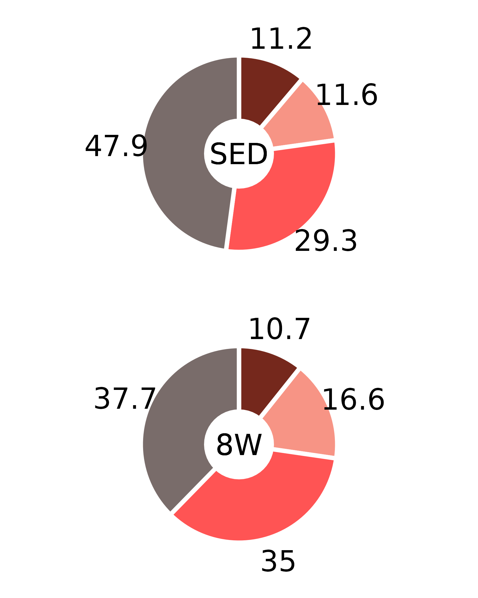
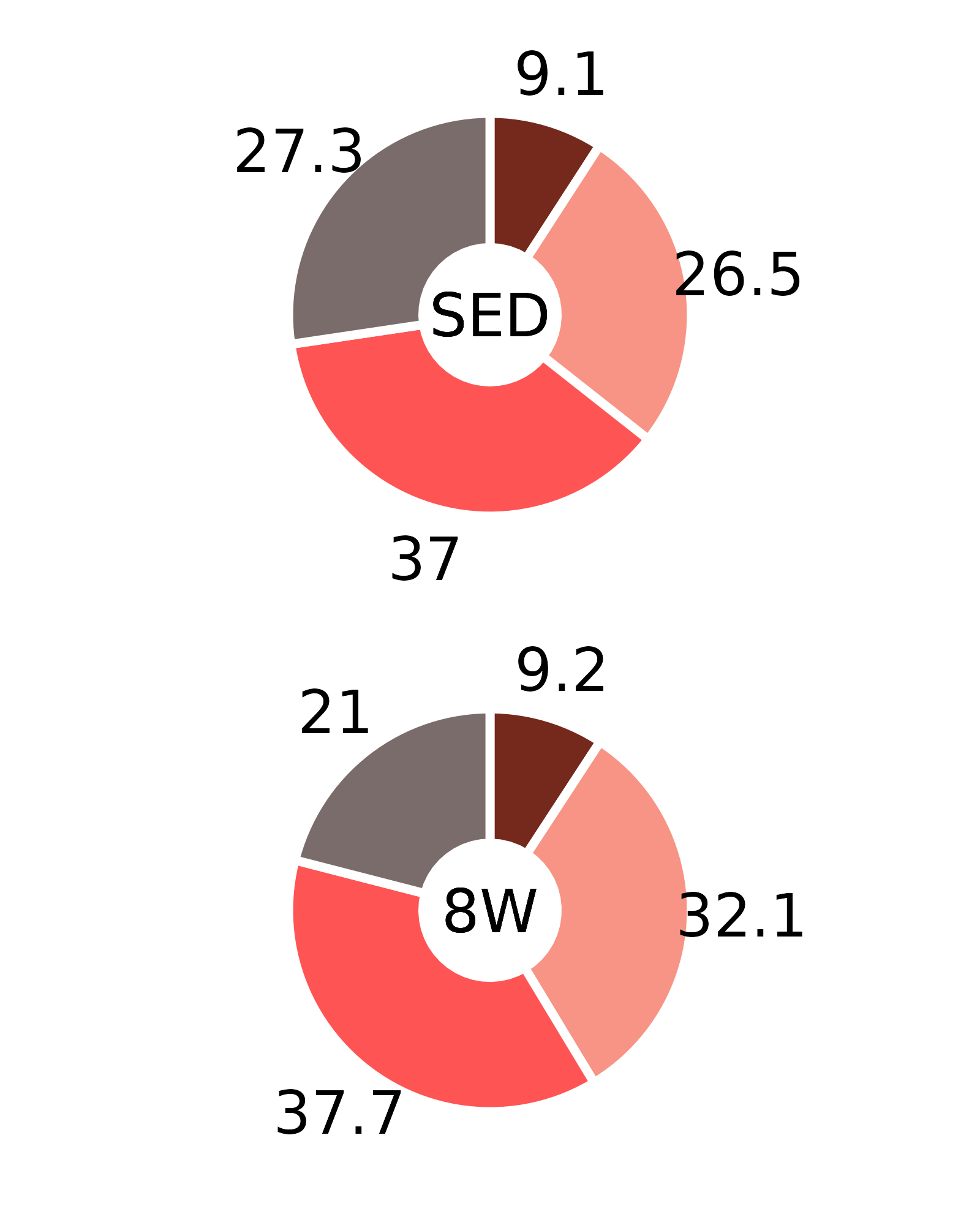
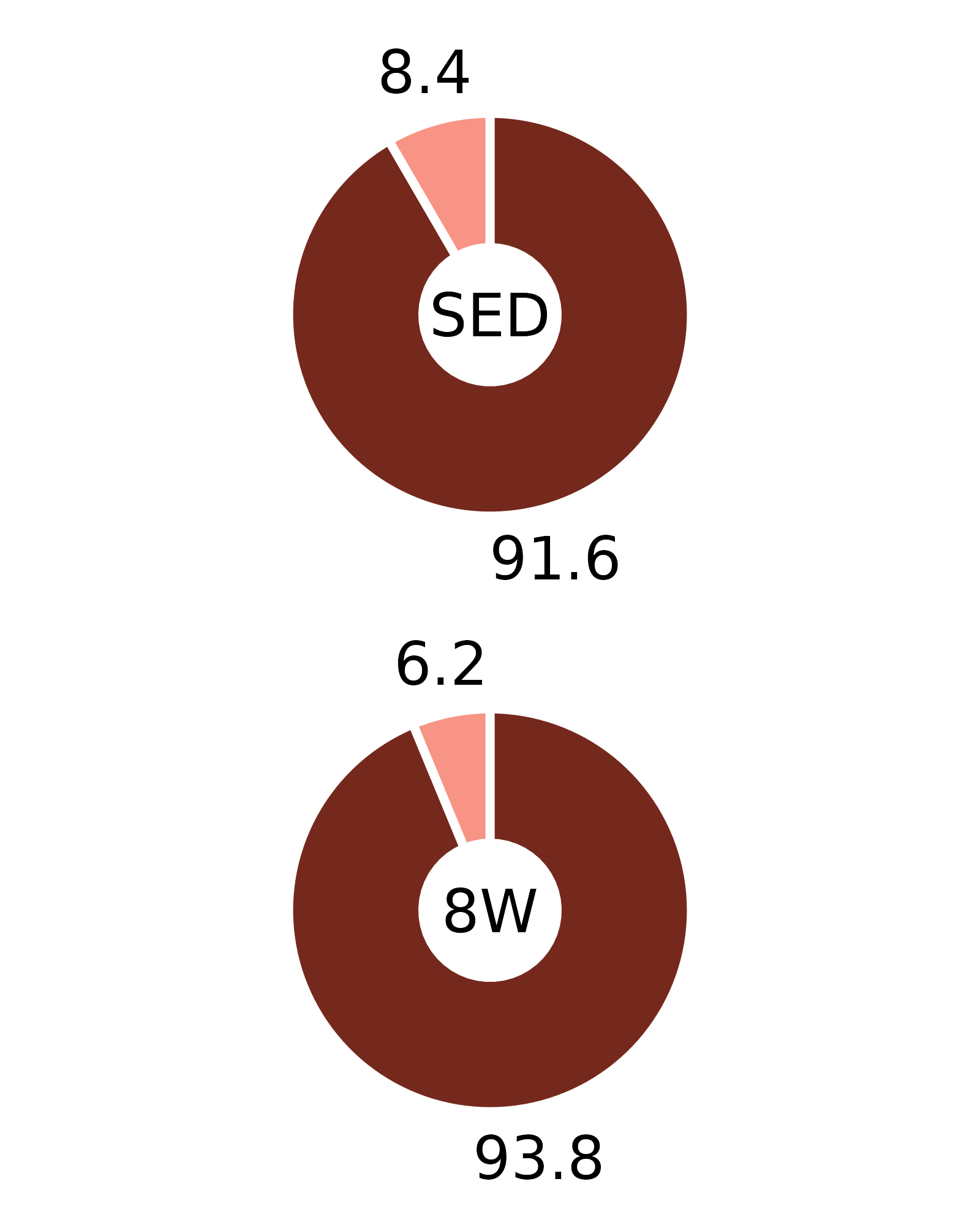
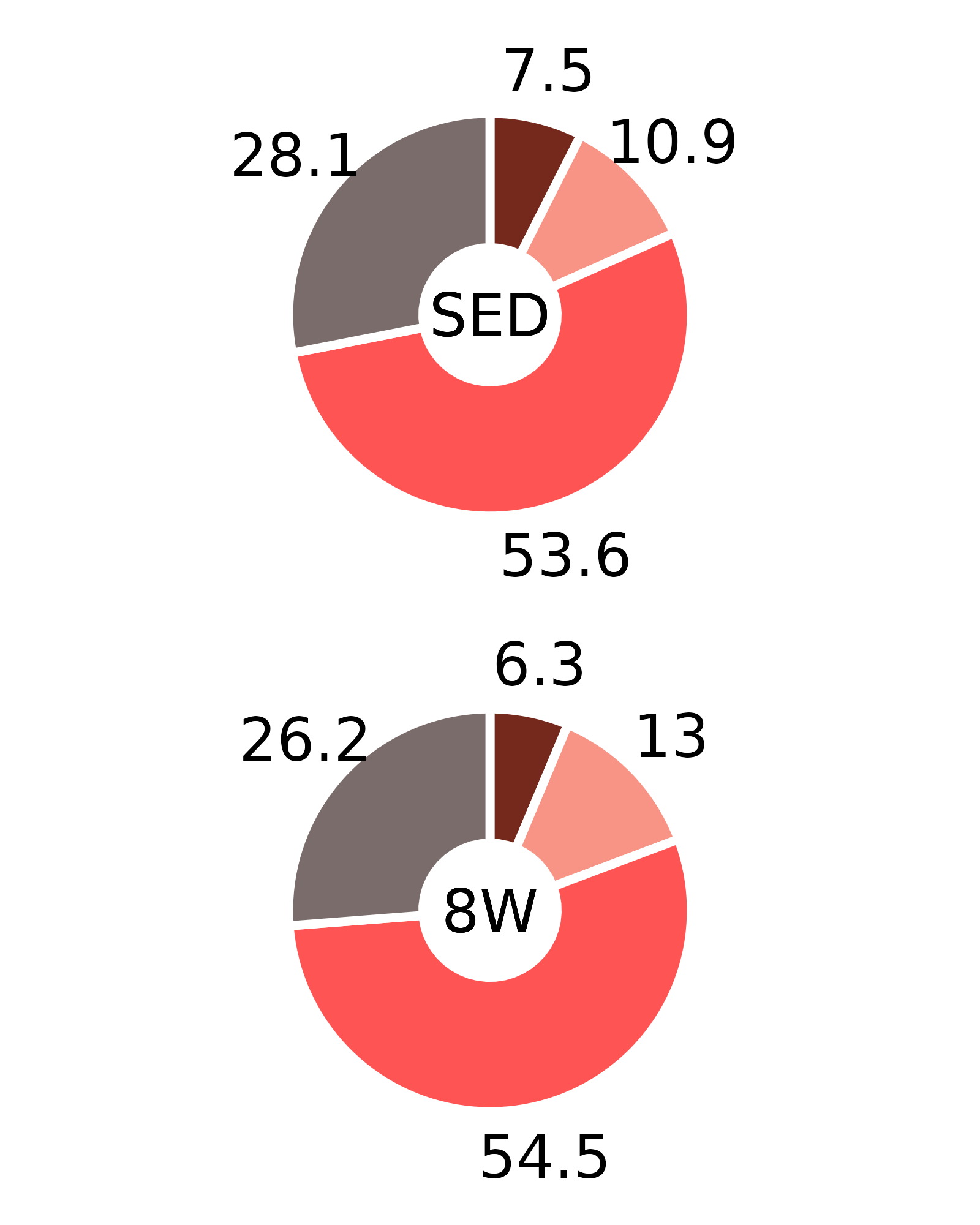
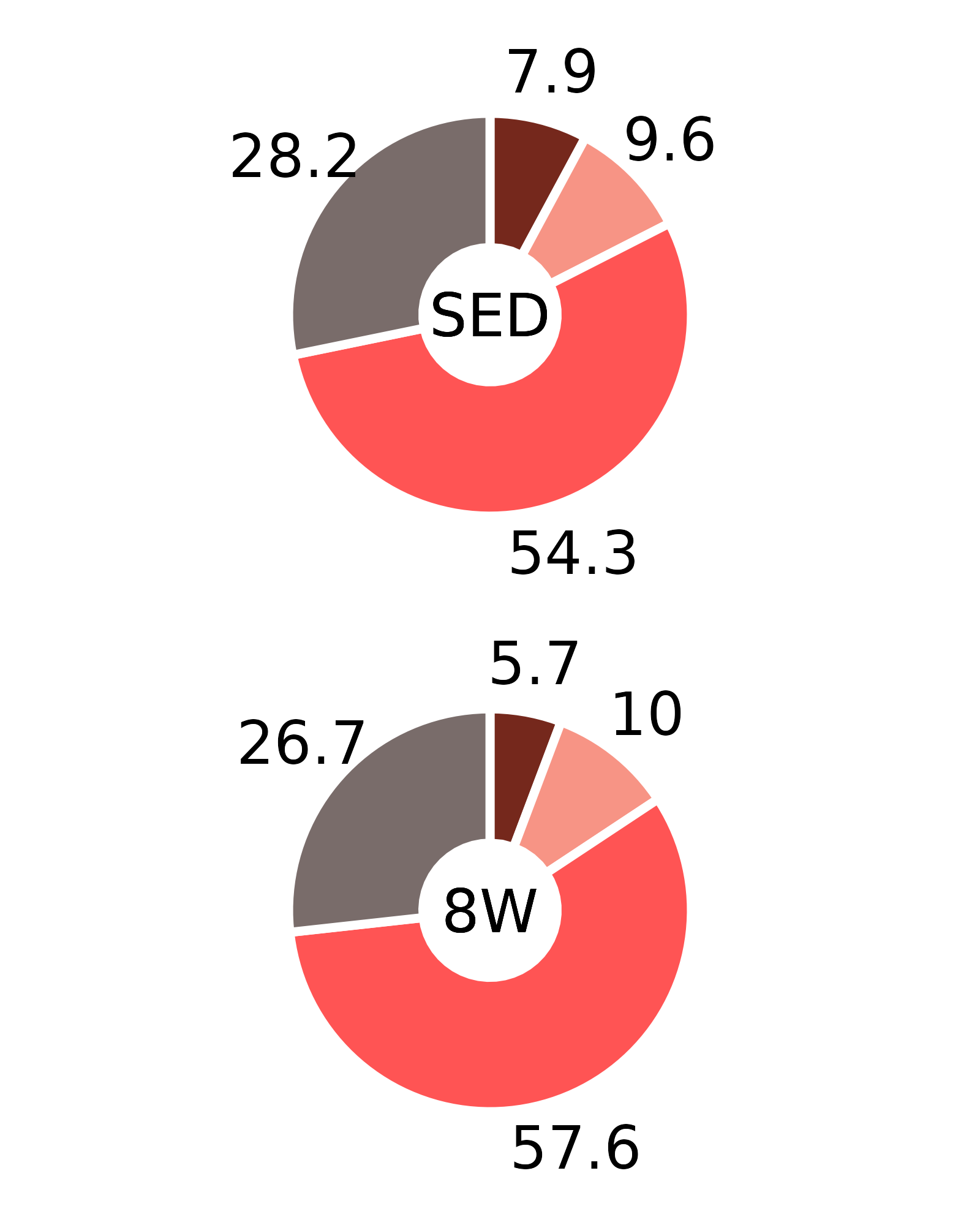
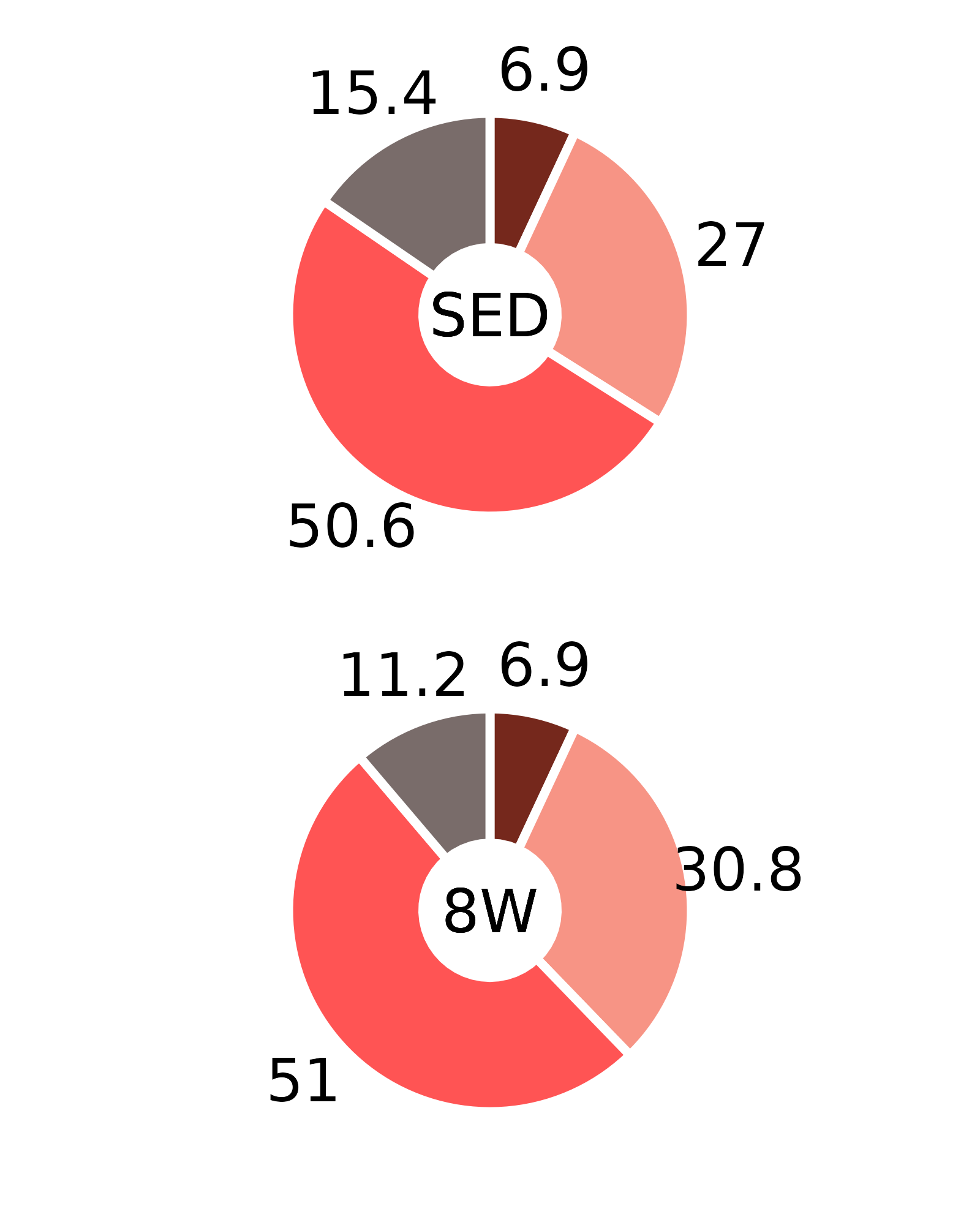
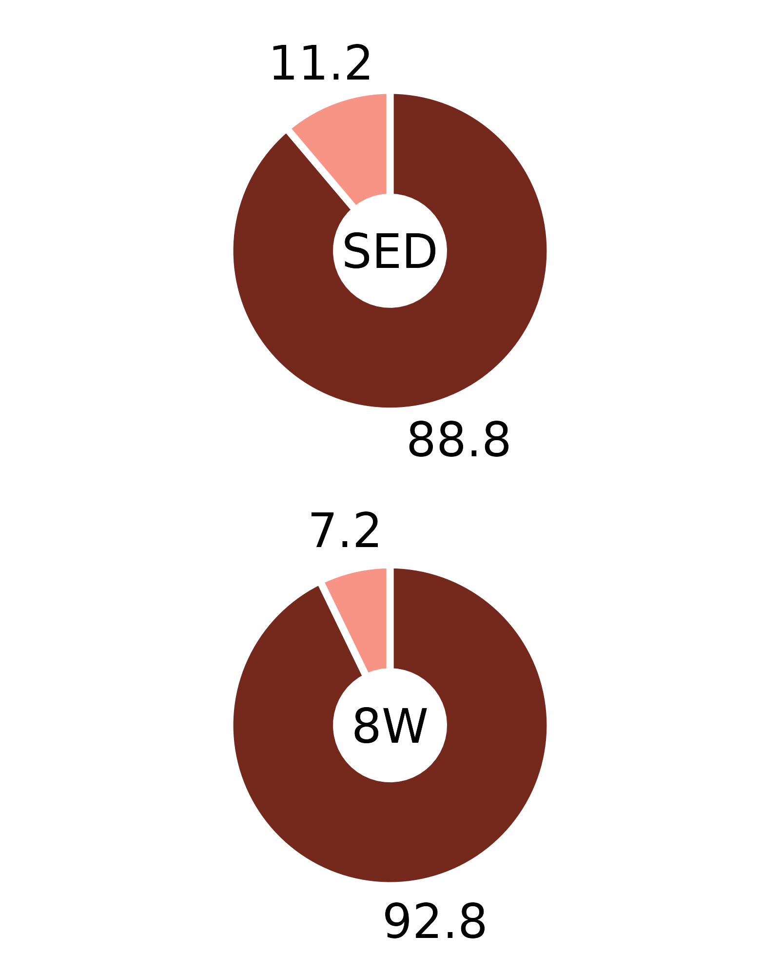
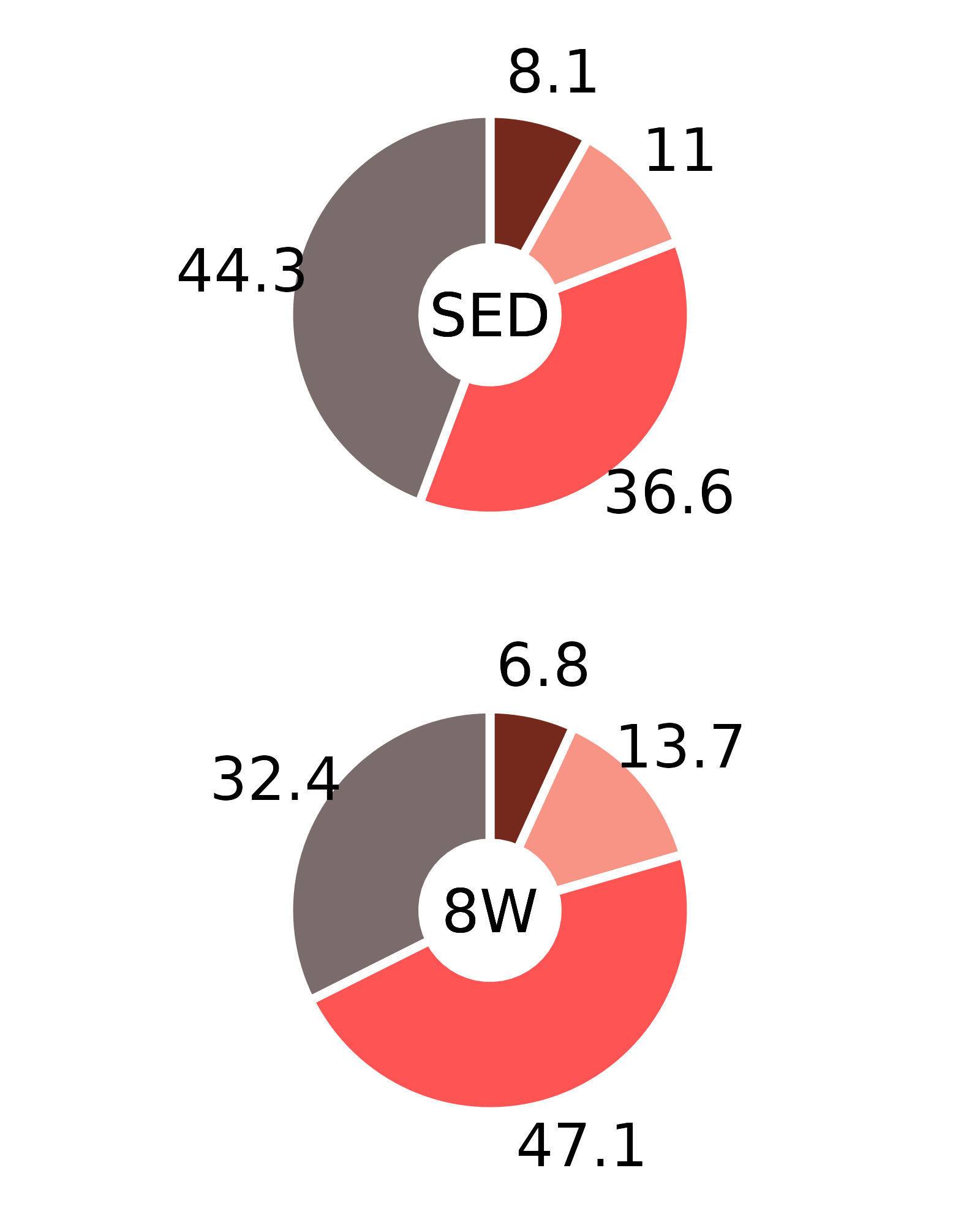
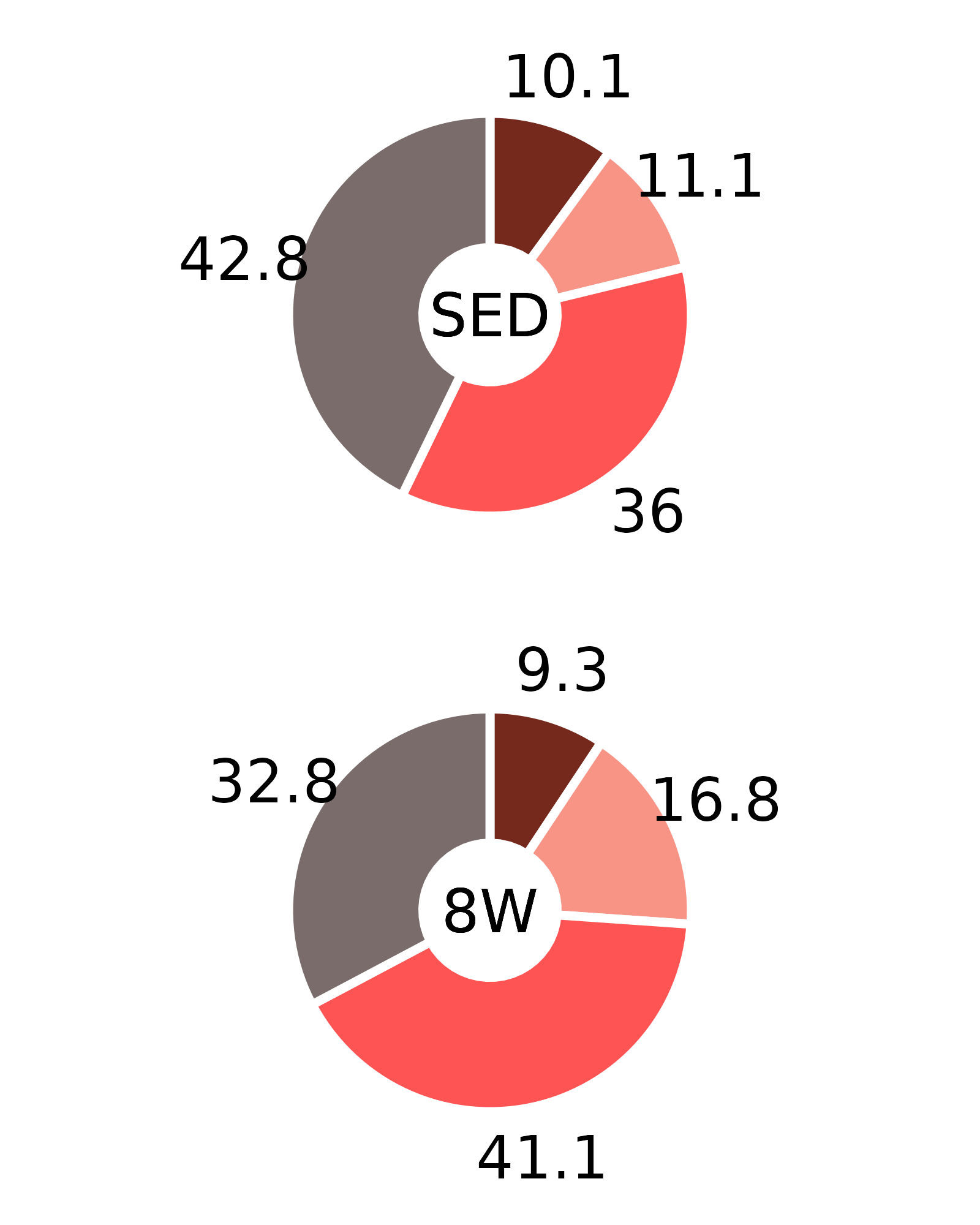
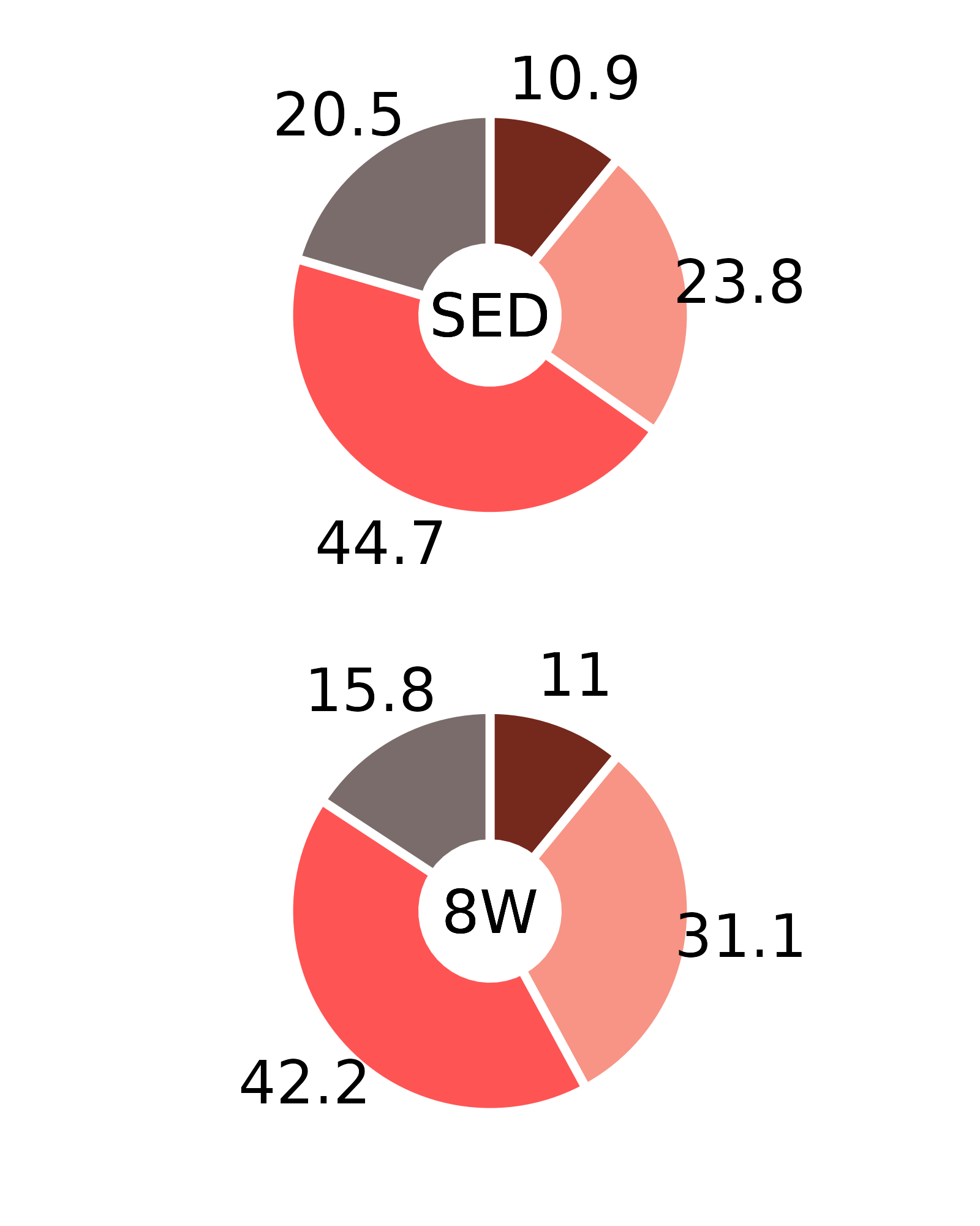
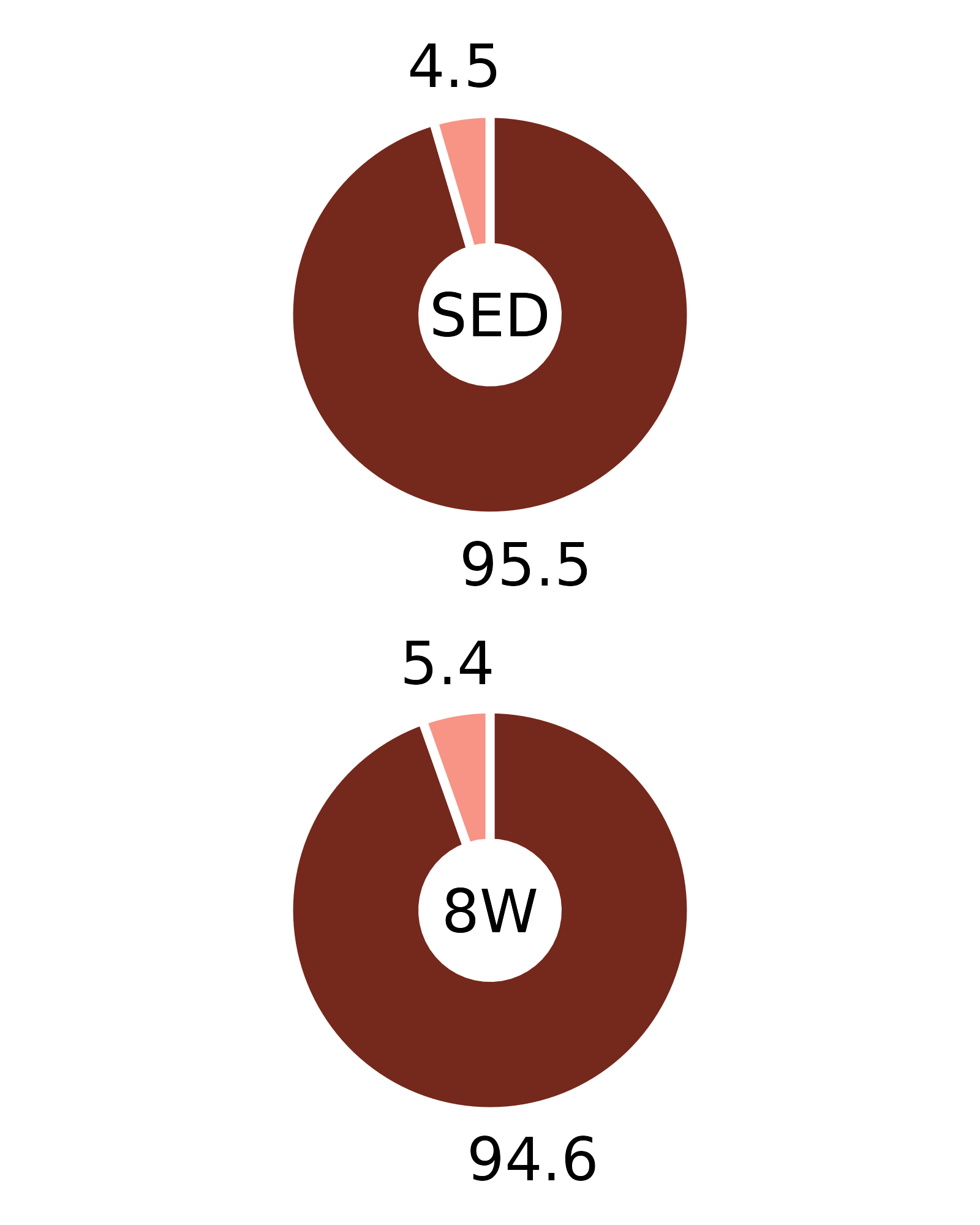
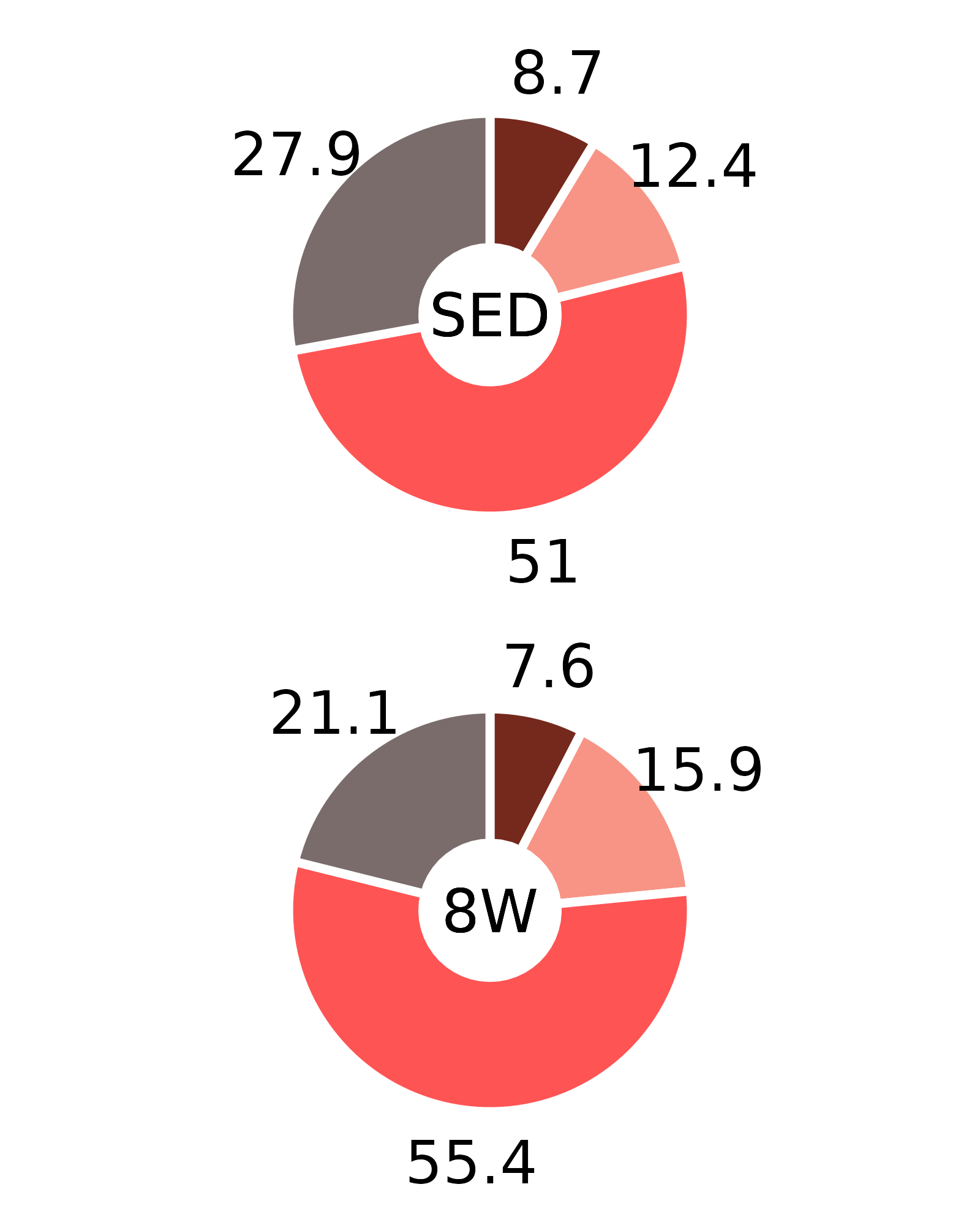
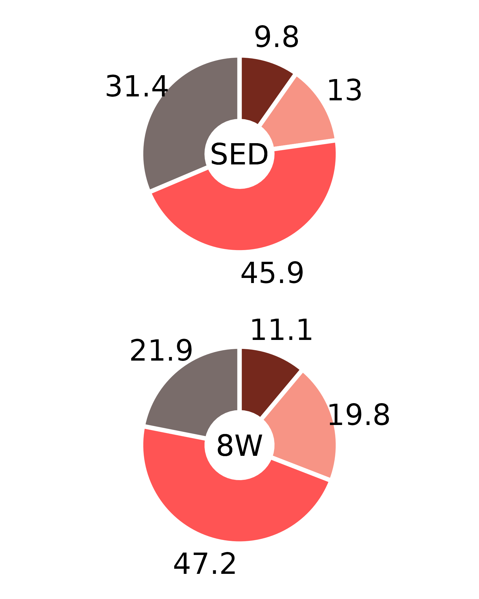
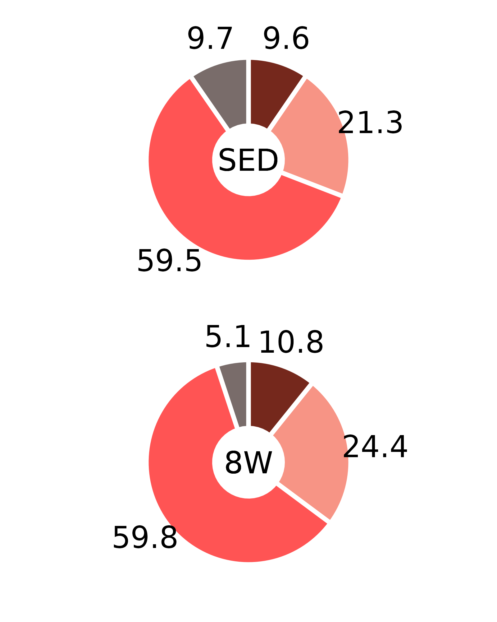
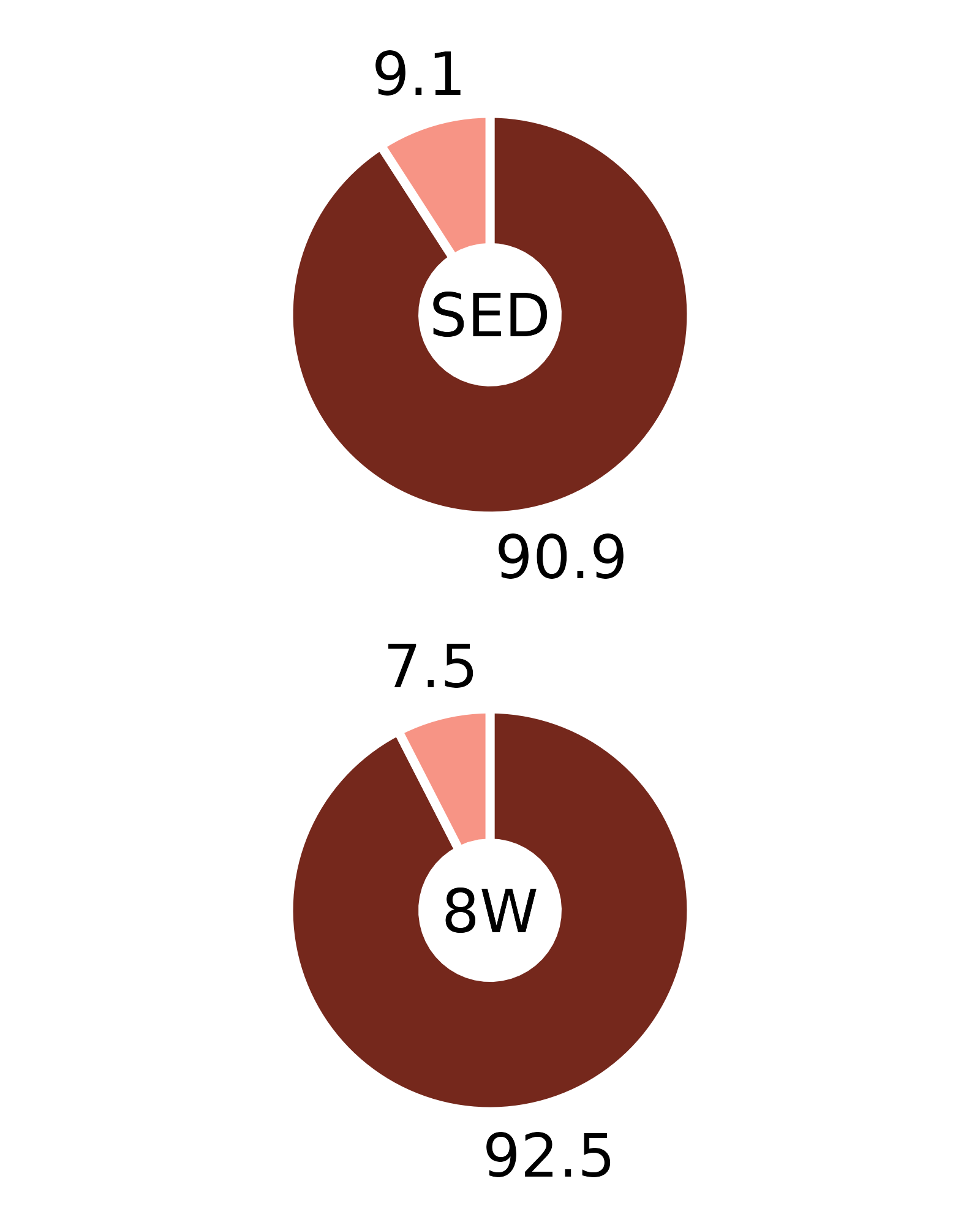
This article generates plots of the mean fiber type percentages. These values are calculated by summing the fiber counts across samples within each age, sex, group, and fiber type combination and dividing by the total fiber count and then multiplying by 100%. The percentage symbols (%) are not displayed on the plots to save space. Since there is no need to specify different y-axes, we can create and save all 16 plots with a few lines of code. Please refer to the “Statistical analysis of fiber counts by muscle and fiber type” vignette for details of the statistical analyses (not shown on the plots due to the complexity of the comparisons).

# Create all plots
foo <- FIBER_TYPES %>% 
  nest(.by = c(age, sex, muscle)) %>% 
  mutate(plots = map(.x = data, .f = fiber_donut_chart),
         file_name = file.path("..", "..", "plots",
                               sprintf("fiber_count_%s_%s_%s.pdf", 
                                       muscle, age, tolower(sex))))

# Save all plots
map2(.x = foo$file_name, .y = foo$plots, 
     .f = ~ ggsave(filename = .x, plot = .y, 
                   height = 2, width = 1.3,
                   family = "ArialMT"))

# Add legend back to plots for display and to save legend separately
foo <- foo %>% 
  mutate(plots = map(.x = plots, .f = ~ .x + theme(legend.position = "right")))

# Save legend
lgd <- get_legend(p = foo$plots[[1]]) %>% 
  as_ggplot()

ggsave(filename = file.path("..", "..", "plots", "fiber_count_legend.pdf"),
       plot = lgd, height = 0.7, width = 0.4, family = "ArialMT")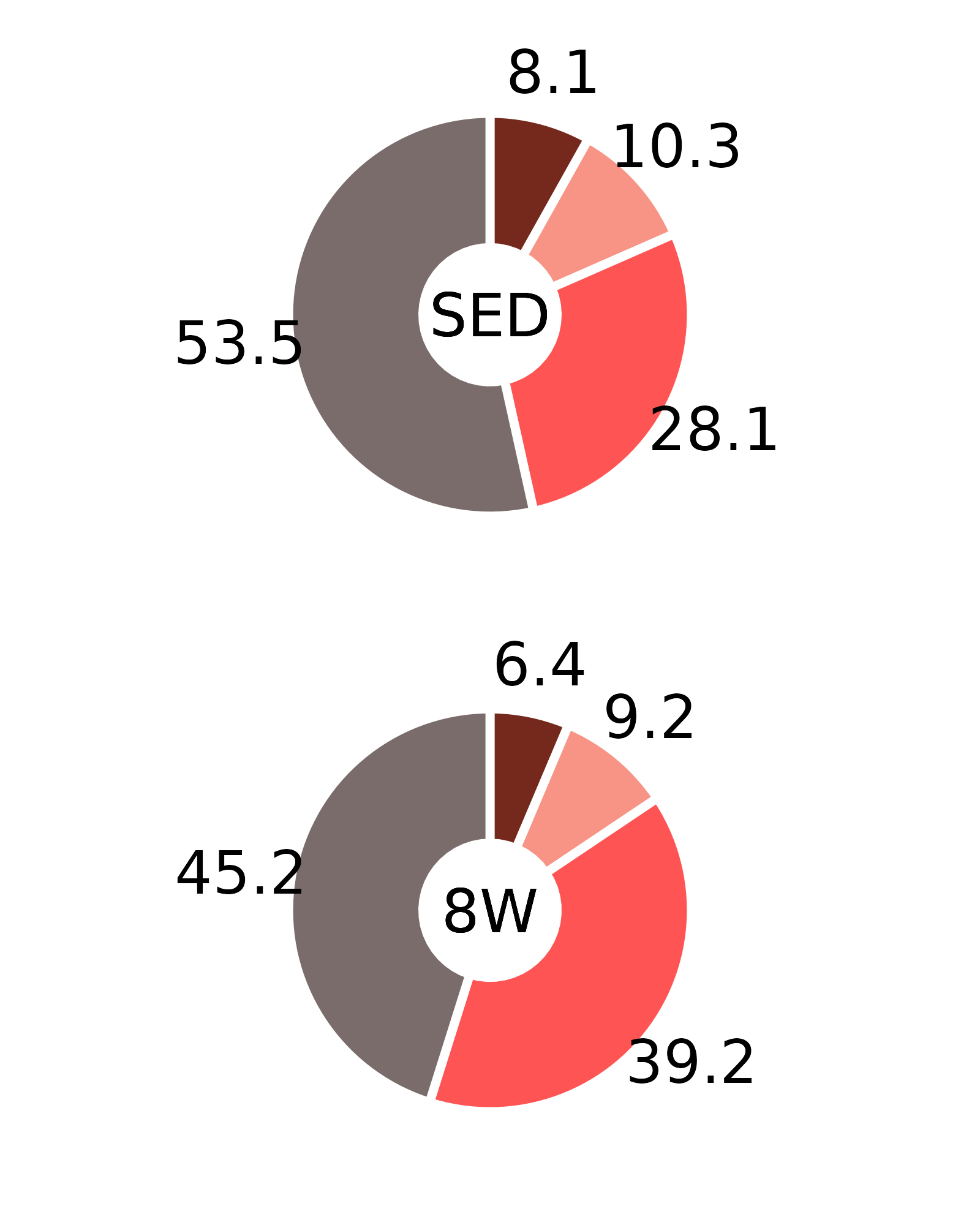

6M Female

LG

foo %>% 
  filter(age == "6M", sex == "Female", muscle == "LG") %>%
  pull(plots) %>% 
  .[[1]]

MG

foo %>% 
  filter(age == "6M", sex == "Female", muscle == "MG") %>% 
  pull(plots) %>% 
  .[[1]]

PL

foo %>% 
  filter(age == "6M", sex == "Female", muscle == "PL") %>% 
  pull(plots) %>% 
  .[[1]]

SOL

foo %>% 
  filter(age == "6M", sex == "Female", muscle == "SOL") %>% 
  pull(plots) %>% 
  .[[1]]

6M Male

LG

foo %>% 
  filter(age == "6M", sex == "Male", muscle == "LG") %>% 
  pull(plots) %>% 
  .[[1]]

MG

foo %>% 
  filter(age == "6M", sex == "Male", muscle == "MG") %>% 
  pull(plots) %>% 
  .[[1]]

PL

foo %>% 
  filter(age == "6M", sex == "Male", muscle == "PL") %>% 
  pull(plots) %>% 
  .[[1]]

SOL

foo %>% 
  filter(age == "6M", sex == "Male", muscle == "SOL") %>% 
  pull(plots) %>% 
  .[[1]]

18M Female

LG

foo %>% 
  filter(age == "18M", sex == "Female", muscle == "LG") %>% 
  pull(plots) %>% 
  .[[1]]

MG

foo %>% 
  filter(age == "18M", sex == "Female", muscle == "MG") %>% 
  pull(plots) %>% 
  .[[1]]

PL

foo %>% 
  filter(age == "18M", sex == "Female", muscle == "PL") %>% 
  pull(plots) %>% 
  .[[1]]

SOL

foo %>% 
  filter(age == "18M", sex == "Female", muscle == "SOL") %>% 
  pull(plots) %>% 
  .[[1]]

18M Male

LG

foo %>% 
  filter(age == "18M", sex == "Male", muscle == "LG") %>% 
  pull(plots) %>% 
  .[[1]]

MG

foo %>% 
  filter(age == "18M", sex == "Male", muscle == "MG") %>% 
  pull(plots) %>% 
  .[[1]]

PL

foo %>% 
  filter(age == "18M", sex == "Male", muscle == "PL") %>% 
  pull(plots) %>% 
  .[[1]]

SOL

foo %>% 
  filter(age == "18M", sex == "Male", muscle == "SOL") %>% 
  pull(plots) %>% 
  .[[1]]

Session Info

sessionInfo()
#> R version 4.4.0 (2024-04-24)
#> Platform: x86_64-pc-linux-gnu
#> Running under: Ubuntu 22.04.4 LTS
#> 
#> Matrix products: default
#> BLAS:   /usr/lib/x86_64-linux-gnu/openblas-pthread/libblas.so.3 
#> LAPACK: /usr/lib/x86_64-linux-gnu/openblas-pthread/libopenblasp-r0.3.20.so;  LAPACK version 3.10.0
#> 
#> locale:
#>  [1] LC_CTYPE=C.UTF-8       LC_NUMERIC=C           LC_TIME=C.UTF-8       
#>  [4] LC_COLLATE=C.UTF-8     LC_MONETARY=C.UTF-8    LC_MESSAGES=C.UTF-8   
#>  [7] LC_PAPER=C.UTF-8       LC_NAME=C              LC_ADDRESS=C          
#> [10] LC_TELEPHONE=C         LC_MEASUREMENT=C.UTF-8 LC_IDENTIFICATION=C   
#> 
#> time zone: UTC
#> tzcode source: system (glibc)
#> 
#> attached base packages:
#> [1] stats     graphics  grDevices utils     datasets  methods   base     
#> 
#> other attached packages:
#> [1] purrr_1.0.2                           
#> [2] tidyr_1.3.1                           
#> [3] ggplot2_3.5.1                         
#> [4] dplyr_1.1.4                           
#> [5] MotrpacRatTrainingPhysiologyData_2.0.0
#> 
#> loaded via a namespace (and not attached):
#>  [1] sass_0.4.9        utf8_1.2.4        generics_0.1.3    rstatix_0.7.2    
#>  [5] digest_0.6.35     magrittr_2.0.3    evaluate_0.23     grid_4.4.0       
#>  [9] fastmap_1.1.1     jsonlite_1.8.8    backports_1.4.1   fansi_1.0.6      
#> [13] scales_1.3.0      textshaping_0.3.7 jquerylib_0.1.4   abind_1.4-5      
#> [17] cli_3.6.2         rlang_1.1.3       munsell_0.5.1     withr_3.0.0      
#> [21] cachem_1.0.8      yaml_2.3.8        ggbeeswarm_0.7.2  tools_4.4.0      
#> [25] memoise_2.0.1     ggsignif_0.6.4    colorspace_2.1-0  ggpubr_0.6.0     
#> [29] broom_1.0.5       vctrs_0.6.5       R6_2.5.1          lifecycle_1.0.4  
#> [33] fs_1.6.4          car_3.1-2         htmlwidgets_1.6.4 vipor_0.4.7      
#> [37] ragg_1.3.0        pkgconfig_2.0.3   beeswarm_0.4.0    desc_1.4.3       
#> [41] pkgdown_2.0.9     pillar_1.9.0      bslib_0.7.0       gtable_0.3.5     
#> [45] glue_1.7.0        systemfonts_1.0.6 highr_0.10        xfun_0.43        
#> [49] tibble_3.2.1      tidyselect_1.2.1  knitr_1.46        farver_2.1.1     
#> [53] htmltools_0.5.8.1 labeling_0.4.3    rmarkdown_2.26    carData_3.0-5    
#> [57] compiler_4.4.0

Tyler Sagendorf

01 May, 2024