Statistical analysis of mean fiber area by muscle and fiber type
Tyler Sagendorf
01 May, 2024
Source:vignettes/FIBER_AREA_STATS.Rmd
FIBER_AREA_STATS.Rmd
# Required packages
library(MotrpacRatTrainingPhysiologyData)
library(ggplot2)
library(MASS)
library(dplyr)
library(tibble)
library(tidyr)
library(purrr)
library(emmeans)
library(nlme)
library(stats)
theme_set(theme_bw()) # base plot theme
Plots
We will look at plots of mean fiber area.
MG
# Plot points
FIBER_TYPES %>%
  filter(muscle == "MG") %>%
  ggplot(aes(x = group, y = fiber_area)) +
  geom_point(na.rm = TRUE, alpha = 0.5,
             position = position_jitter(width = 0.1, height = 0)) +
  facet_grid(age + sex ~ type)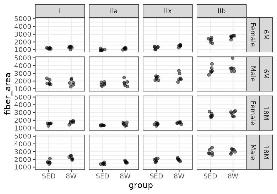
LG
# Plot points
FIBER_TYPES %>%
  filter(muscle == "LG") %>%
  ggplot(aes(x = group, y = fiber_area)) +
  geom_point(na.rm = TRUE, alpha = 0.5,
             position = position_jitter(width = 0.1, height = 0)) +
  facet_grid(age + sex ~ type)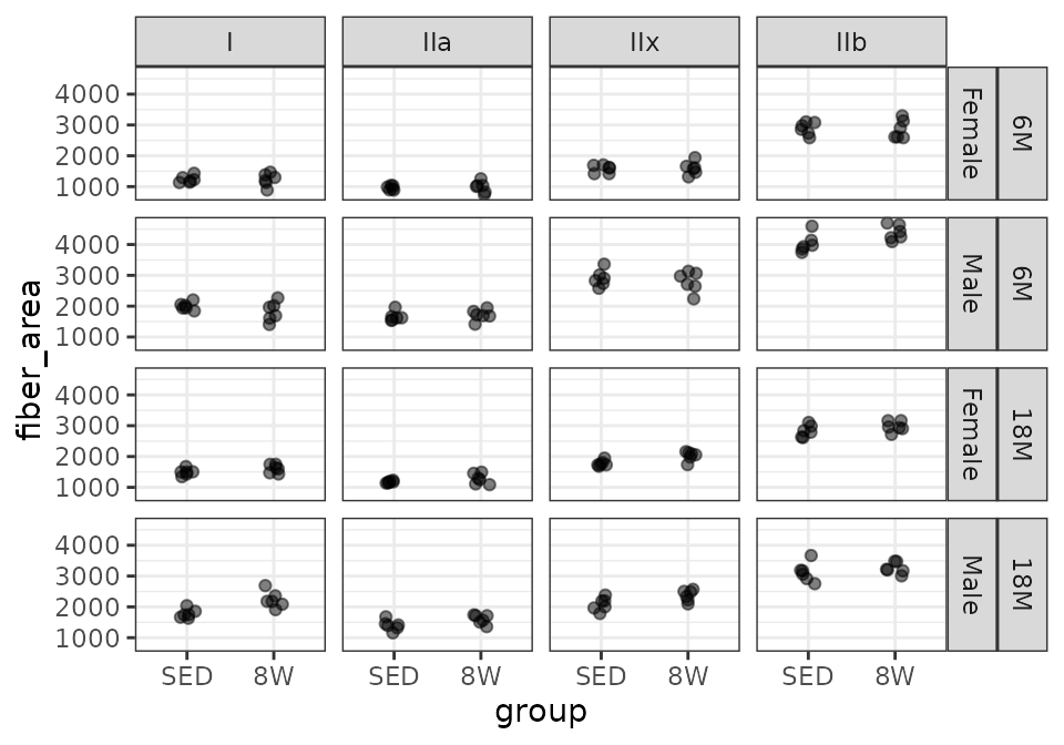
PL
# Plot points
FIBER_TYPES %>%
  filter(muscle == "PL") %>%
  ggplot(aes(x = group, y = fiber_area)) +
  geom_point(na.rm = TRUE, alpha = 0.5,
             position = position_jitter(width = 0.1, height = 0)) +
  facet_grid(age + sex ~ type)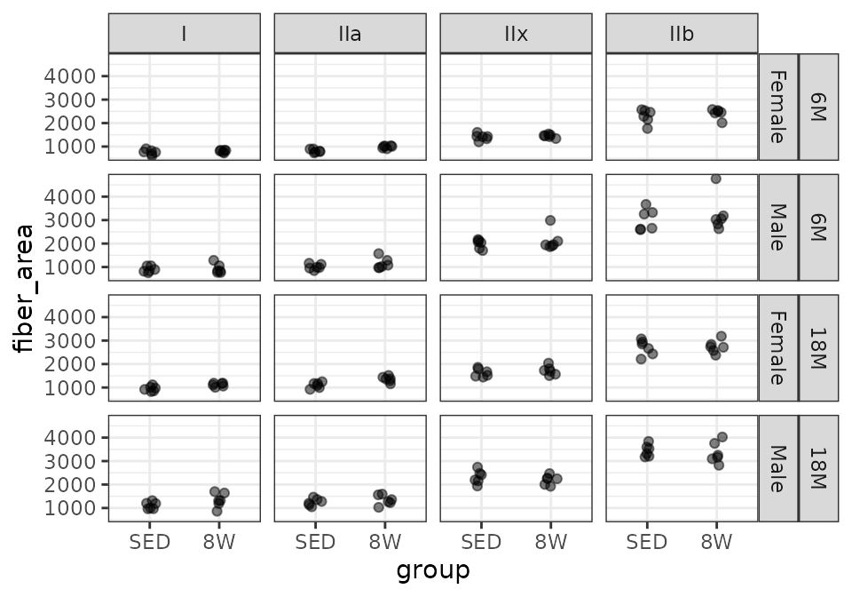
SOL
# Plot points
FIBER_TYPES %>%
  filter(muscle == "SOL") %>%
  ggplot(aes(x = group, y = fiber_area)) +
  geom_point(na.rm = TRUE, alpha = 0.5,
             position = position_jitter(width = 0.1, height = 0)) +
  facet_grid(age + sex ~ type)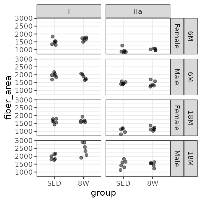
Regression Models
We will check the mean-variance relationship.
mv <- FIBER_TYPES %>%
  group_by(sex, group, age, muscle, type) %>%
  summarise(mn = mean(fiber_area, na.rm = TRUE),
            vr = var(fiber_area, na.rm = TRUE))

fit.mv <- lm(log(vr) ~ log(mn), data = mv)
coef(fit.mv)
#> (Intercept)     log(mn)
#>   -4.451949    1.982954
plot(log(vr) ~ log(mn), data = mv, las = 1, pch = 19,
     xlab = "log(group means)", ylab = "log(group variances)")
abline(coef(fit.mv), lwd = 2)
The slope of the line is close to 2, which suggests a gamma
distribution or log transformation may be appropriate. Since SOL only
consists of type I and IIa fibers, we can not include an interaction
between muscle and type, since it will be
inestimable for SOL type IIb and IIx. Instead, we will create a new
muscle_type variable by concatenating muscle
and type.
FIBER_TYPES <- mutate(FIBER_TYPES, muscle_type = paste0(muscle, ".", type))

fit.area <- lme(fixed = log(fiber_area) ~ age * sex * group * muscle_type,
                random = ~ 1 | pid,
                data = FIBER_TYPES,
                na.action = na.exclude)
We will check regression diagnostic plots and plots of residuals vs. predictor levels.
r <- resid(fit.area, scaled = TRUE, type = "pearson")

par(mfrow = c(2, 2))
# Standardized residuals vs. fitted plot
plot(x = fitted(fit.area), y = r,
     ylab = "Standardized residuals", xlab = "Fitted values")
lines(loess.smooth(x = fitted(fit.area), y = r, degree = 2),
      col = "red", lwd = 2)

# Scale-location plot
plot(x = fitted(fit.area), y = sqrt(abs(r)),
     ylab = "sqrt(|standardized residuals|)", xlab = "Fitted values")
lines(loess.smooth(x = fitted(fit.area), y = sqrt(abs(r)), degree = 2),
      col = "red", lwd = 2)

# Normal Q-Q plot
qqnorm(r); qqline(r, col = "red")
par(mfrow = c(1, 1))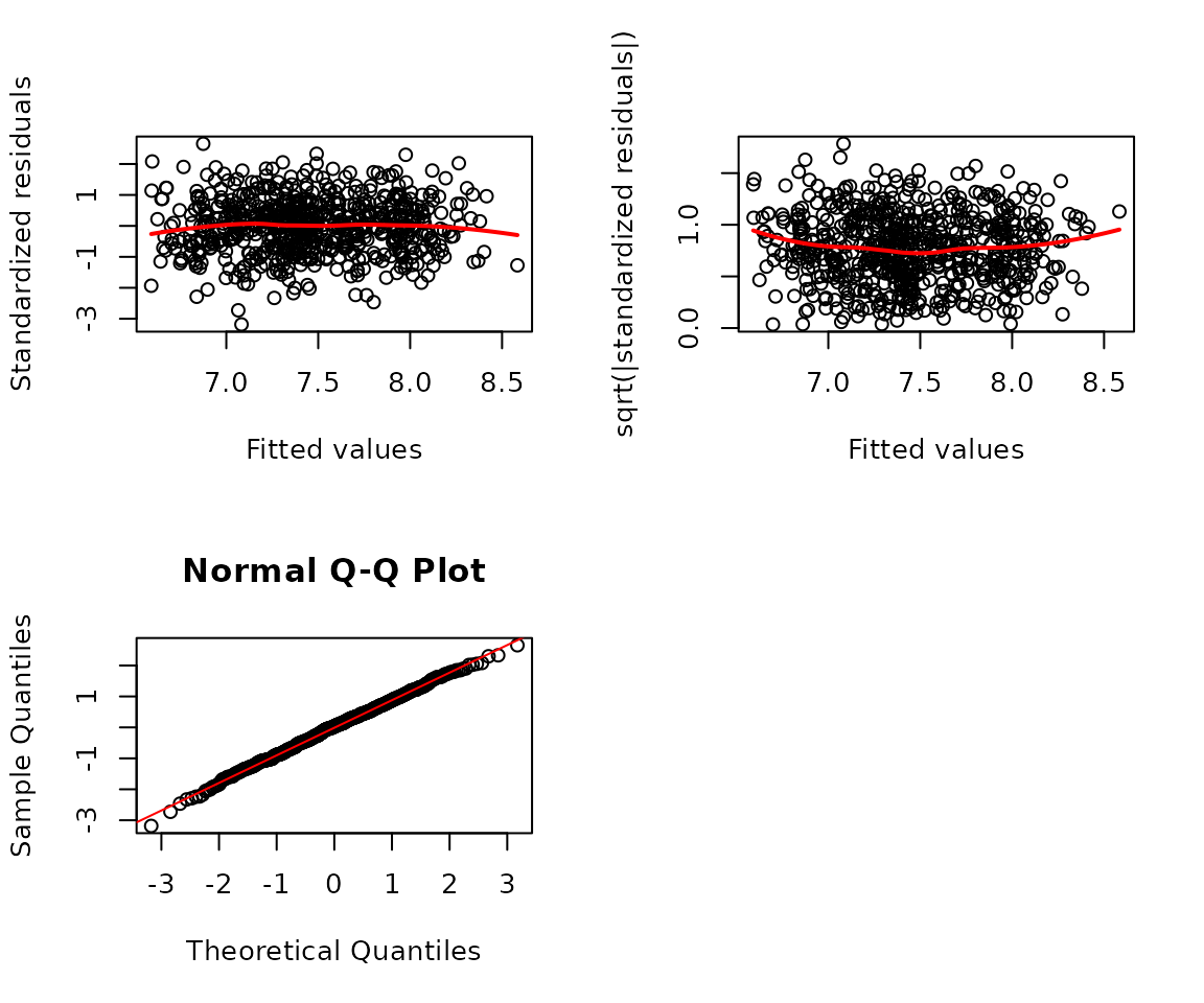
# Residuals vs. predictor levels
par(mfrow = c(2, 3), mar = c(5, 3, 0.5, 0.5))
boxplot(r ~ age, data = FIBER_TYPES, ylab = "")
boxplot(r ~ group, data = FIBER_TYPES, ylab = "")
boxplot(r ~ sex, data = FIBER_TYPES, ylab = "")
boxplot(r ~ muscle, data = FIBER_TYPES, ylab = "")
boxplot(r ~ type, data = FIBER_TYPES, ylab = "")
mtext("Standardized residuals", side = 2, line = -1, outer = TRUE)
par(mfrow = c(1, 1), mar = c(5, 4, 4, 2))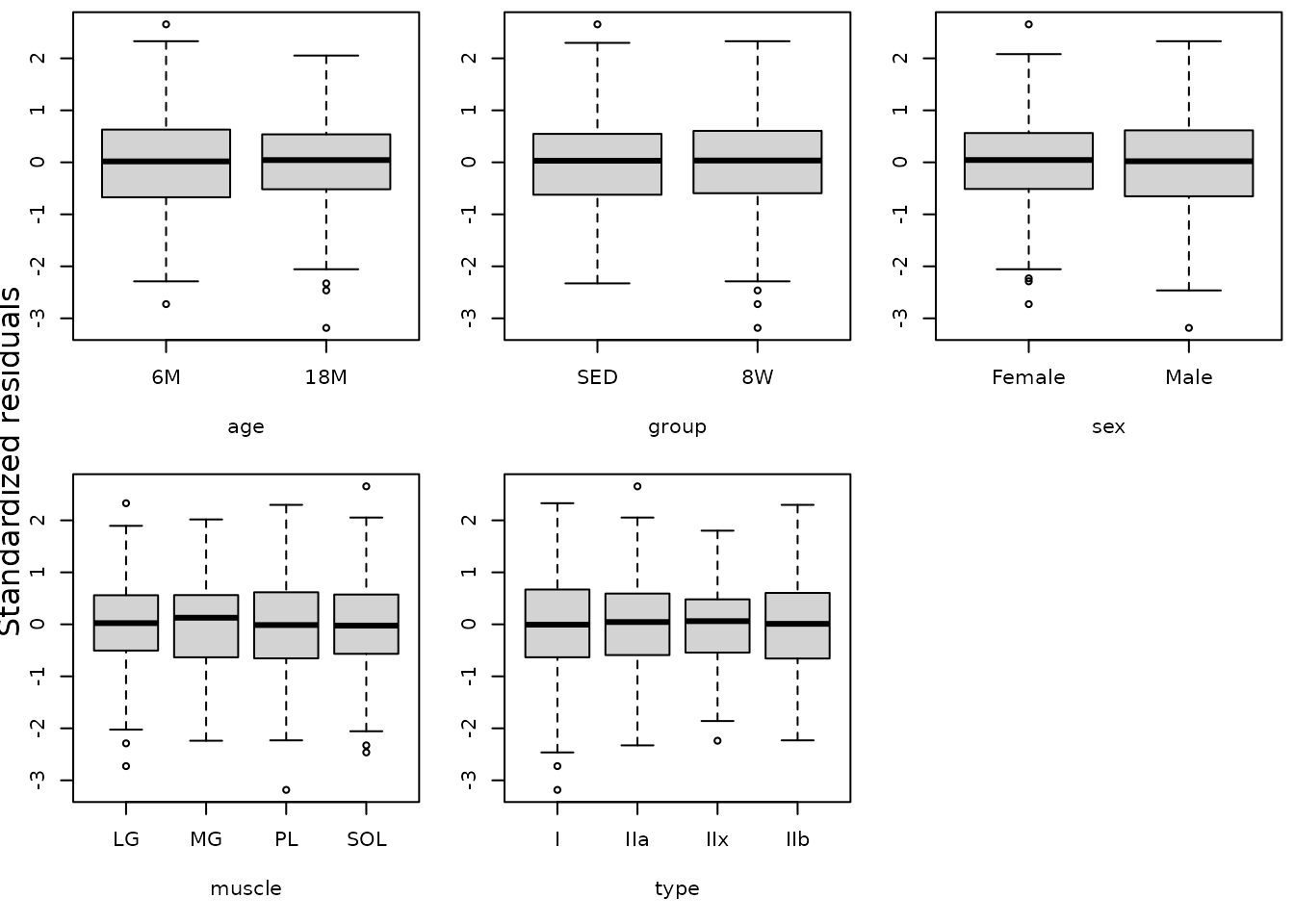
The diagnostic plots look fine.
anova(fit.area)
#>                           numDF denDF  F-value p-value
#> (Intercept)                   1   518 594342.4  <.0001
#> age                           1    40     19.9  0.0001
#> sex                           1    40    207.9  <.0001
#> group                         1    40     15.2  0.0004
#> muscle_type                  13   518    632.1  <.0001
#> age:sex                       1    40     26.3  <.0001
#> age:group                     1    40      1.5  0.2338
#> sex:group                     1    40      0.5  0.5025
#> age:muscle_type              13   518     15.5  <.0001
#> sex:muscle_type              13   518      8.3  <.0001
#> group:muscle_type            13   518      1.8  0.0451
#> age:sex:group                 1    40      0.8  0.3873
#> age:sex:muscle_type          13   518      7.7  <.0001
#> age:group:muscle_type        13   518      2.6  0.0017
#> sex:group:muscle_type        13   518      0.9  0.5899
#> age:sex:group:muscle_type    13   518      1.6  0.0821
VarCorr(fit.area)
#> pid = pdLogChol(1)
#>             Variance    StdDev
#> (Intercept) 0.003757709 0.06130015
#> Residual    0.010165279 0.10082301
Hypothesis Testing
We will compare the 8W trained to the sedentary control group within each age, sex, and muscle using a two-sided t-test. We will then adjust p-values across fiber types within each age, sex, and muscle group using the Holm method.
# Estimated marginal means
FIBER_AREA_EMM <- emmeans(fit.area, specs = "group",
                          by = c("age", "sex", "muscle_type"),
                          type = "response", infer = TRUE)
# Extract model info
model_df <- data.frame(response = "Mean Fiber Area",
                       model = paste(deparse(fit.area[["call"]]),
                                     collapse = "")) %>%
  mutate(model = gsub("(?<=[\\s])\\s*|^\\s+|\\s+$", "", model, perl = TRUE),
         model_type = "lme",
         fixed = sub(".*fixed = ([^,]+),.*", "\\1", model),
         random = "~1 | pid") %>%
  dplyr::select(-model)
FIBER_AREA_STATS <- FIBER_AREA_EMM %>%
  contrast(method = "trt.vs.ctrl") %>%
  summary(infer = TRUE) %>%
  as.data.frame() %>%
  rename(any_of(c(lower.CL = "asymp.LCL",
                  upper.CL = "asymp.UCL"))) %>%
  separate_wider_delim(cols = muscle_type, delim = ".",
                       names = c("muscle", "type")) %>%
  mutate(muscle = factor(muscle, levels = c("LG", "MG", "PL", "SOL")),
         type = factor(type, levels = c("I", "IIa", "IIx", "IIb"))) %>%
  # Holm-adjust p-values across fiber types within each age, sex, and muscle
  # combination
  group_by(age, sex, muscle) %>%
  mutate(p.adj = p.adjust(p.value, method = "holm"),
         signif = p.adj < 0.05) %>%
  ungroup() %>%
  pivot_longer(cols = ratio,
               names_to = "estimate_type",
               values_to = "estimate",
               values_drop_na = TRUE) %>%
  pivot_longer(cols = contains(".ratio"),
               names_to = "statistic_type",
               values_to = "statistic",
               values_drop_na = TRUE) %>%
  mutate(response = "Mean Fiber Area",
         statistic_type = sub("\\.ratio", "", statistic_type)) %>%
  left_join(model_df, by = "response") %>%
  # Reorder columns
  dplyr::select(response, age, sex, muscle, type, contrast, estimate_type, null,
                estimate, SE, lower.CL, upper.CL, statistic_type, statistic,
                df, p.value, p.adj, signif, model_type, fixed, random,
                everything()) %>%
  arrange(response, age, sex, muscle, type) %>%
  as.data.frame()
See ?FIBER_AREA_STATS for details.
print.data.frame(head(FIBER_AREA_STATS))
#>          response age    sex muscle type contrast estimate_type null  estimate
#> 1 Mean Fiber Area  6M Female     LG    I 8W / SED         ratio    1 0.9858807
#> 2 Mean Fiber Area  6M Female     LG  IIa 8W / SED         ratio    1 1.0077985
#> 3 Mean Fiber Area  6M Female     LG  IIx 8W / SED         ratio    1 1.0069759
#> 4 Mean Fiber Area  6M Female     LG  IIb 8W / SED         ratio    1 0.9865055
#> 5 Mean Fiber Area  6M Female     MG    I 8W / SED         ratio    1 1.0947372
#> 6 Mean Fiber Area  6M Female     MG  IIa 8W / SED         ratio    1 1.1627512
#>           SE  lower.CL upper.CL statistic_type  statistic df   p.value
#> 1 0.06716298 0.8590696 1.131411              t -0.2087328 40 0.8357162
#> 2 0.06865613 0.8781682 1.156564              t  0.1140301 40 0.9097843
#> 3 0.06860009 0.8774514 1.155620              t  0.1020439 40 0.9192317
#> 4 0.06720554 0.8596140 1.132128              t -0.1994340 40 0.8429336
#> 5 0.07457881 0.9539241 1.256336              t  1.3286536 40 0.1914926
#> 6 0.07921226 1.0131897 1.334390              t  2.2134207 40 0.0326355
#>        p.adj signif model_type
#> 1 1.00000000  FALSE        lme
#> 2 1.00000000  FALSE        lme
#> 3 1.00000000  FALSE        lme
#> 4 1.00000000  FALSE        lme
#> 5 0.19149264  FALSE        lme
#> 6 0.06527099  FALSE        lme
#>                                               fixed   random
#> 1 log(fiber_area) ~ age * sex * group * muscle_type ~1 | pid
#> 2 log(fiber_area) ~ age * sex * group * muscle_type ~1 | pid
#> 3 log(fiber_area) ~ age * sex * group * muscle_type ~1 | pid
#> 4 log(fiber_area) ~ age * sex * group * muscle_type ~1 | pid
#> 5 log(fiber_area) ~ age * sex * group * muscle_type ~1 | pid
#> 6 log(fiber_area) ~ age * sex * group * muscle_type ~1 | pid
Session Info
sessionInfo()
#> R version 4.4.0 (2024-04-24)
#> Platform: x86_64-pc-linux-gnu
#> Running under: Ubuntu 22.04.4 LTS
#>
#> Matrix products: default
#> BLAS:   /usr/lib/x86_64-linux-gnu/openblas-pthread/libblas.so.3
#> LAPACK: /usr/lib/x86_64-linux-gnu/openblas-pthread/libopenblasp-r0.3.20.so;  LAPACK version 3.10.0
#>
#> locale:
#>  [1] LC_CTYPE=C.UTF-8       LC_NUMERIC=C           LC_TIME=C.UTF-8
#>  [4] LC_COLLATE=C.UTF-8     LC_MONETARY=C.UTF-8    LC_MESSAGES=C.UTF-8
#>  [7] LC_PAPER=C.UTF-8       LC_NAME=C              LC_ADDRESS=C
#> [10] LC_TELEPHONE=C         LC_MEASUREMENT=C.UTF-8 LC_IDENTIFICATION=C
#>
#> time zone: UTC
#> tzcode source: system (glibc)
#>
#> attached base packages:
#> [1] stats     graphics  grDevices utils     datasets  methods   base
#>
#> other attached packages:
#> [1] nlme_3.1-164
#> [2] emmeans_1.10.1
#> [3] purrr_1.0.2
#> [4] tidyr_1.3.1
#> [5] tibble_3.2.1
#> [6] dplyr_1.1.4
#> [7] MASS_7.3-60.2
#> [8] ggplot2_3.5.1
#> [9] MotrpacRatTrainingPhysiologyData_2.0.0
#>
#> loaded via a namespace (and not attached):
#>  [1] sass_0.4.9        utf8_1.2.4        generics_0.1.3    rstatix_0.7.2
#>  [5] stringi_1.8.3     lattice_0.22-6    digest_0.6.35     magrittr_2.0.3
#>  [9] estimability_1.5  evaluate_0.23     grid_4.4.0        mvtnorm_1.2-4
#> [13] fastmap_1.1.1     jsonlite_1.8.8    backports_1.4.1   fansi_1.0.6
#> [17] scales_1.3.0      textshaping_0.3.7 jquerylib_0.1.4   abind_1.4-5
#> [21] cli_3.6.2         rlang_1.1.3       munsell_0.5.1     withr_3.0.0
#> [25] cachem_1.0.8      yaml_2.3.8        ggbeeswarm_0.7.2  tools_4.4.0
#> [29] memoise_2.0.1     ggsignif_0.6.4    colorspace_2.1-0  ggpubr_0.6.0
#> [33] broom_1.0.5       vctrs_0.6.5       R6_2.5.1          lifecycle_1.0.4
#> [37] stringr_1.5.1     fs_1.6.4          car_3.1-2         htmlwidgets_1.6.4
#> [41] vipor_0.4.7       ragg_1.3.0        pkgconfig_2.0.3   beeswarm_0.4.0
#> [45] desc_1.4.3        pkgdown_2.0.9     pillar_1.9.0      bslib_0.7.0
#> [49] gtable_0.3.5      glue_1.7.0        systemfonts_1.0.6 highr_0.10
#> [53] xfun_0.43         tidyselect_1.2.1  knitr_1.46        farver_2.1.1
#> [57] htmltools_0.5.8.1 labeling_0.4.3    rmarkdown_2.26    carData_3.0-5
#> [61] compiler_4.4.0