Plots of weekly body mass and blood lactate
Tyler Sagendorf
01 May, 2024
Source:vignettes/articles/weekly_measures_plots.Rmd
weekly_measures_plots.Rmd
# Required packages
library(MotrpacRatTrainingPhysiologyData)
library(dplyr)
library(ggplot2)
library(tidyr)
library(emmeans)
library(latex2exp)
Weekly Body Mass
Body mass (g) was measured at the start of each week prior to training.
6M Female
WEEKLY_BODY_MASS_EMM %>%
  summary(type = "response", infer = TRUE) %>%
  as.data.frame() %>%
  dplyr::rename(week = week,
                response_mean = response) %>%
  filter(age == "6M", sex == "Female") %>%
  ggplot(aes(x = week, y = response_mean)) +
  geom_crossbar(aes(ymin = lower.CL, ymax = upper.CL),
                fatten = 1, color = "#ff6eff",
                width = 0.7, linewidth = 0.4) +
  facet_grid(~ group) +
  scale_y_continuous(name = "Body Mass (g)",
                     expand = expansion(mult = 5e-3),
                     breaks = seq(180, 250, 20)) +
  coord_cartesian(ylim = c(175, 255), clip = "off") +
  labs(x = "Week") +
  theme_bw(base_size = 7) +
  theme(text = element_text(color = "black"),
        axis.text = element_text(color = "black", size = 7),
        axis.title = element_text(color = "black", size = 7),
        axis.ticks = element_line(color = "black"),
        axis.ticks.x = element_blank(),
        strip.text = element_text(color = "black", size = 7),
        strip.background = element_blank(),
        panel.spacing = unit(-1, "pt"),
        panel.grid = element_blank())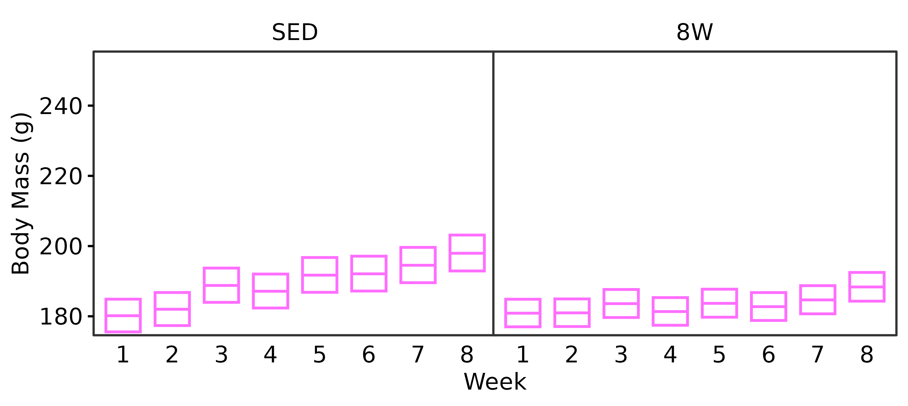
6M Male
WEEKLY_BODY_MASS_EMM %>%
  summary(type = "response", infer = TRUE) %>%
  as.data.frame() %>%
  filter(age == "6M", sex == "Male") %>%
  dplyr::rename(week = week,
                response_mean = response) %>%
  ggplot(aes(x = week, y = response_mean)) +
  geom_crossbar(aes(ymin = lower.CL, ymax = upper.CL),
                fatten = 1, color = "#5555ff",
                width = 0.7, linewidth = 0.4) +
  facet_grid(~ group) +
  scale_y_continuous(name = "Body Mass (g)",
                     breaks = seq(300, 440, 40),
                     expand = expansion(mult = 5e-3)) +
  coord_cartesian(ylim = c(300, 450), clip = "off") +
  labs(x = "Week") +
  theme_bw(base_size = 7) +
  theme(text = element_text(color = "black"),
        axis.text = element_text(color = "black", size = 7),
        axis.title = element_text(color = "black", size = 7),
        axis.ticks = element_line(color = "black"),
        axis.ticks.x = element_blank(),
        strip.text = element_text(color = "black", size = 7),
        strip.background = element_blank(),
        panel.spacing = unit(-1, "pt"),
        panel.grid = element_blank())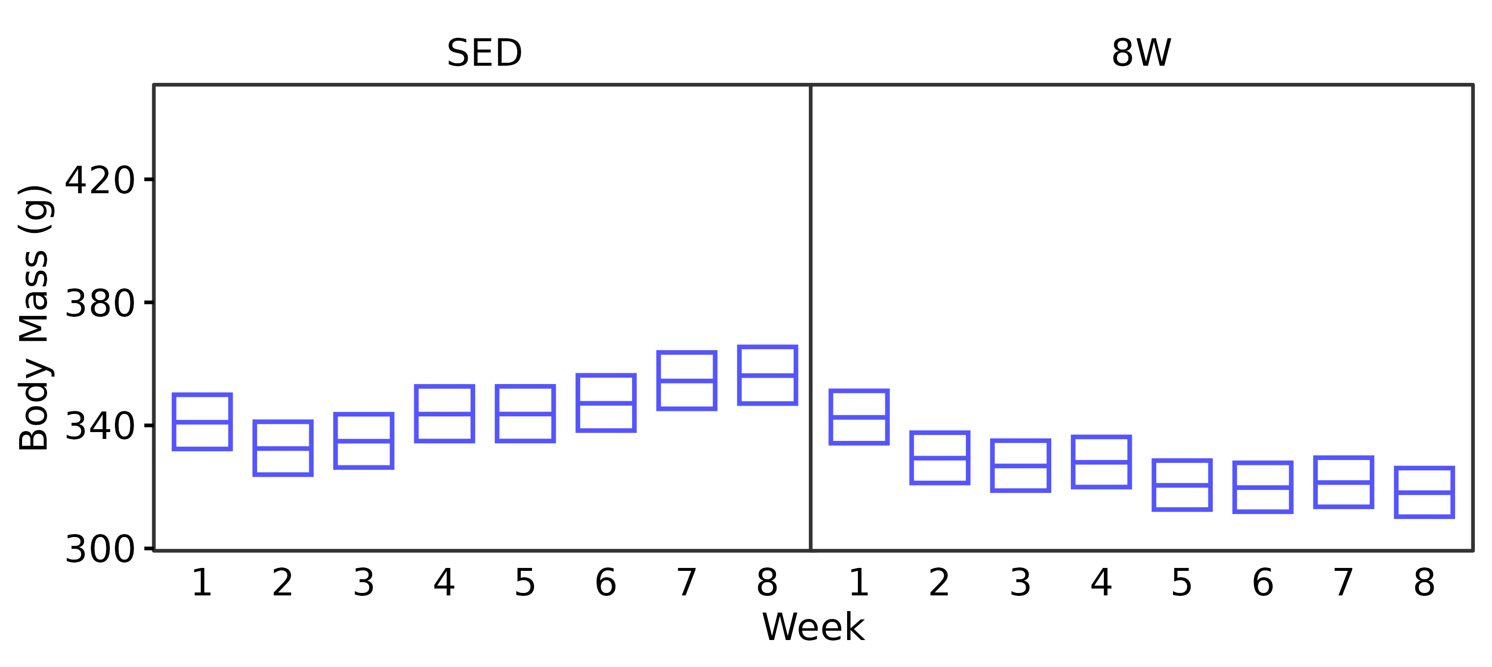
18M Female
WEEKLY_BODY_MASS_EMM %>%
  summary(type = "response", infer = TRUE) %>%
  as.data.frame() %>%
  filter(age == "18M", sex == "Female") %>%
  dplyr::rename(week = week,
                response_mean = response) %>%
  ggplot(aes(x = week, y = response_mean)) +
  geom_crossbar(aes(ymin = lower.CL, ymax = upper.CL),
                fatten = 1, color = "#ff6eff",
                width = 0.7, linewidth = 0.4) +
  facet_grid(~ group) +
  scale_y_continuous(name = "Body Mass (g)",
                     expand = expansion(mult = 5e-3),
                     breaks = seq(180, 250, 20)) +
  coord_cartesian(ylim = c(175, 255), clip = "off") +
  labs(x = "Week") +
  theme_bw(base_size = 7) +
  theme(text = element_text(color = "black"),
        axis.text = element_text(color = "black", size = 7),
        axis.title = element_text(color = "black", size = 7),
        axis.ticks = element_line(color = "black"),
        axis.ticks.x = element_blank(),
        strip.text = element_text(color = "black", size = 7),
        strip.background = element_blank(),
        panel.spacing = unit(-1, "pt"),
        panel.grid = element_blank())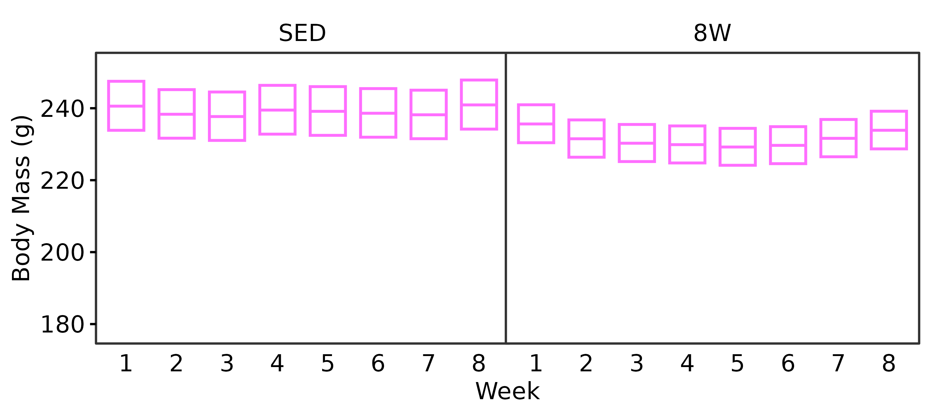
18M Male
WEEKLY_BODY_MASS_EMM %>%
  summary(type = "response", infer = TRUE) %>%
  as.data.frame() %>%
  dplyr::rename(week = week,
                response_mean = response) %>%
  filter(age == "18M", sex == "Male") %>%
  ggplot(aes(x = week, y = response_mean)) +
  geom_crossbar(aes(ymin = lower.CL, ymax = upper.CL),
                fatten = 1, color = "#5555ff",
                width = 0.7, linewidth = 0.4) +
  facet_grid(~ group) +
  scale_y_continuous(name = "Body Mass (g)",
                     breaks = seq(300, 440, 40),
                     expand = expansion(mult = 5e-3)) +
  coord_cartesian(ylim = c(300, 450), clip = "off") +
  labs(x = "Week") +
  theme_bw(base_size = 7) +
  theme(text = element_text(color = "black"),
        axis.text = element_text(color = "black", size = 7),
        axis.title = element_text(color = "black", size = 7),
        axis.ticks = element_line(color = "black"),
        axis.ticks.x = element_blank(),
        strip.text = element_text(color = "black", size = 7),
        strip.background = element_blank(),
        panel.spacing = unit(-1, "pt"),
        panel.grid = element_blank())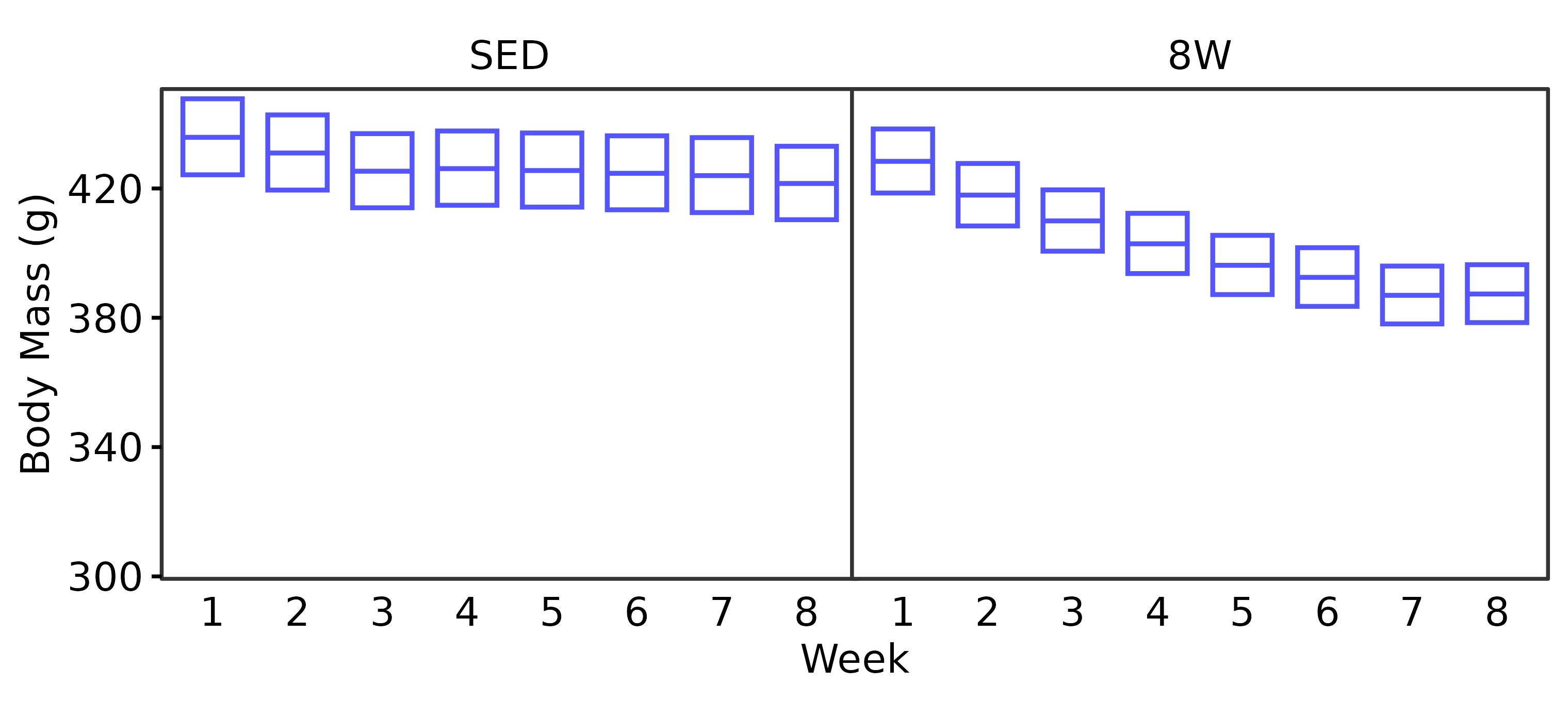
Plot Analysis Results
WEEKLY_BODY_MASS_STATS %>%
  mutate(age = factor(age, levels = c("6M", "18M"),
                      labels = c("Adult", "Aged"))) %>%
  ggplot(aes(x = as.numeric(week), y = estimate, color = sex)) +
  geom_line(aes(x = as.numeric(week), group = sex),
            position = position_dodge(width = 0.5)) +
  geom_errorbar(aes(ymin = lower.CL, ymax = upper.CL,
                    color = sex), width = 0.6, linewidth = 0.5,
                position = position_dodge(width = 0.5)) +
  geom_point(aes(group = sex, shape = signif),
             position = position_dodge(width = 0.5),
             size = 1.5, fill = "white") +
  facet_grid(~ age) +
  geom_hline(yintercept = 1, lty = "dashed") +
  scale_color_manual(values = c("#ff6eff", "#556eff")) +
  scale_shape_manual(name = "Benjamini-Yekutieli-adjusted P-value:",
                     values = c(21, 16),
                     labels = c(latex2exp::TeX("$\\geq 0.05$"), "< 0.05")) +
  guides(color = guide_none()) +
  scale_y_continuous(limits = c(0.85, 1.05),
                     breaks = seq(0.85, 1.05, 0.05),
                     expand = expansion(mult = 5e-3)) +
  labs(x = "Week", y = "8W / SED Mean Ratio") +
  theme_bw(base_size = 7) +
  theme(panel.border = element_rect(color = NA),
        panel.grid = element_blank(),
        axis.line = element_line(color = "black"),
        text = element_text(color = "black"),
        legend.position = "bottom",
        legend.direction = "horizontal",
        legend.margin = margin(t = -2, b = 0),
        legend.key.size = unit(7, "pt"),
        legend.text = element_text(color = "black", size = 7),
        legend.title = element_text(color = "black", size = 7),
        axis.text = element_text(color = "black", size = 7),
        axis.title = element_text(color = "black", size = 7),
        axis.ticks = element_line(color = "black"),
        strip.text = element_text(color = "black", size = 7),
        strip.background = element_blank())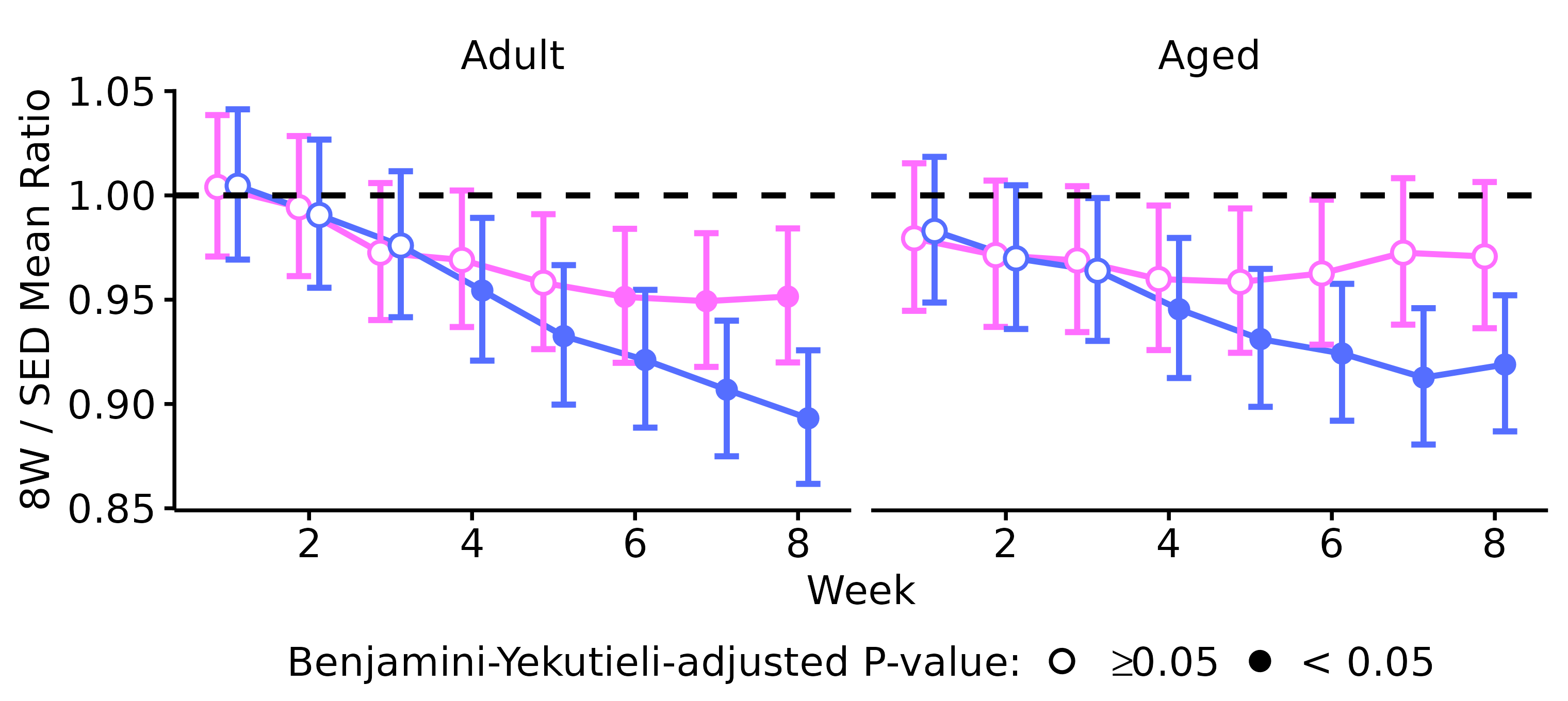
ggsave(filename = file.path("..", "..", "plots", "weekly_body_mass_tests.pdf"),
       height = 2.4, width = 3.8, family = "ArialMT")
Both sexes lose a significant amount of body mass after 3 weeks of exercise. While males continue to lose body mass throughout the protocol, female body mass appears to stabilize starting after 4 weeks of exercise. That is, they experience an initial decrease in body mass that is maintained with training.
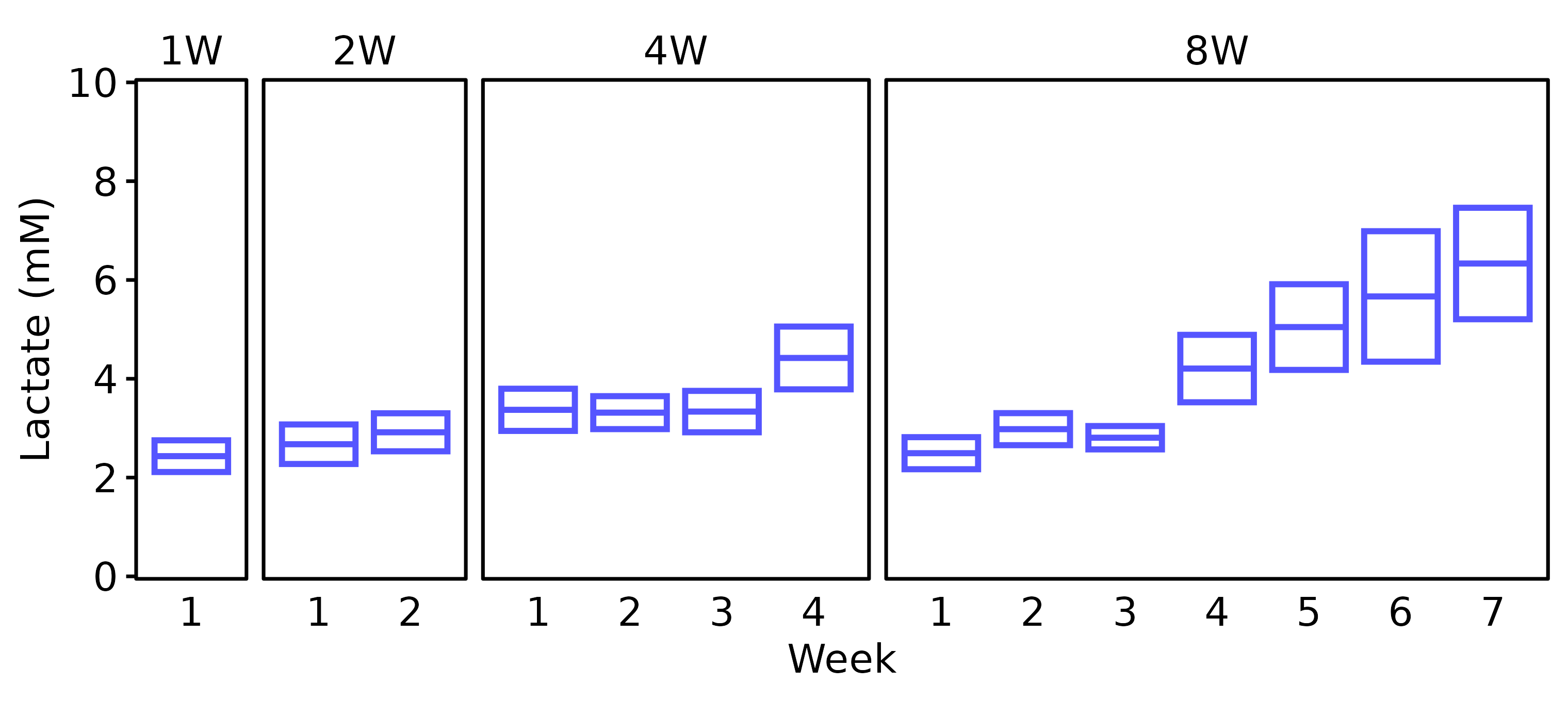
Lactate
Blood lactate was recorded at the start and end of each week at the end of the training bout. For the SED group, blood lactate was only recorded in 18M males, so we will not plot SED values.
lact_df <- WEEKLY_MEASURES %>%
  dplyr::select(pid, age, sex, group, week, week_time, lactate) %>%
  distinct() %>%
  filter(!is.na(lactate)) %>%
  filter(group != "SED") %>%
  mutate(week_time = factor(week_time, levels = c("start", "end"),
                            labels = c("Start", "End")),
         week = factor(week, levels = 1:8, labels = paste0("", 1:8))) %>%
  droplevels.data.frame() %>%
  group_by(age, sex, group, week, week_time) %>%
  mutate(n = n()) %>%
  filter(week_time == "Start")
# Reusable lactate plot code
plot_lactate <- function(x) {
  ggplot() +
    stat_summary(geom = "crossbar", fun.data = mean_cl_normal,
                 data = filter(x, n >= 5),
                 mapping = aes(x = week, y = lactate, color = sex),
                 width = 0.8, linewidth = 0.5, fatten = 1) +
    geom_point(aes(x = week, y = lactate, color = sex),
               data = filter(x, n < 5),
               position = ggbeeswarm::position_beeswarm(cex = 2,
                                                        dodge.width = 0.7),
               shape = 16, size = 0.5) +
    facet_grid(~ group, space = "free", scales = "free") +
    scale_color_manual(values = c("#ff6eff", "#5555ff"),
                       breaks = c("Female", "Male")) +
    labs(x = "Week") +
    theme_bw(base_size = 7) +
    theme(text = element_text(size = 7, color = "black"),
          line = element_line(linewidth = 0.3, color = "black"),
          axis.ticks = element_line(linewidth = 0.3, color = "black"),
          panel.grid = element_blank(),
          panel.border = element_rect(color = "black", fill = NA,
                                      linewidth = 0.3),
          axis.ticks.x = element_blank(),
          axis.text = element_text(size = 7, color = "black"),
          axis.title = element_text(size = 7, margin = margin(),
                                    color = "black"),
          strip.background = element_blank(),
          strip.text = element_text(size = 7, color = "black",
                                    margin = margin(b = 2, t = 2)),
          panel.spacing = unit(3, "pt"),
          legend.position = "none"
    )
}
6M Female
# 6M Female
lact_df %>%
  filter(age == "6M", sex == "Female") %>%
  plot_lactate() +
  scale_y_continuous(name = "Lactate (mM)",
                     expand = expansion(mult = 5e-3),
                     breaks = seq(0, 10, 2)) +
  coord_cartesian(ylim = c(0, 10), clip = "off")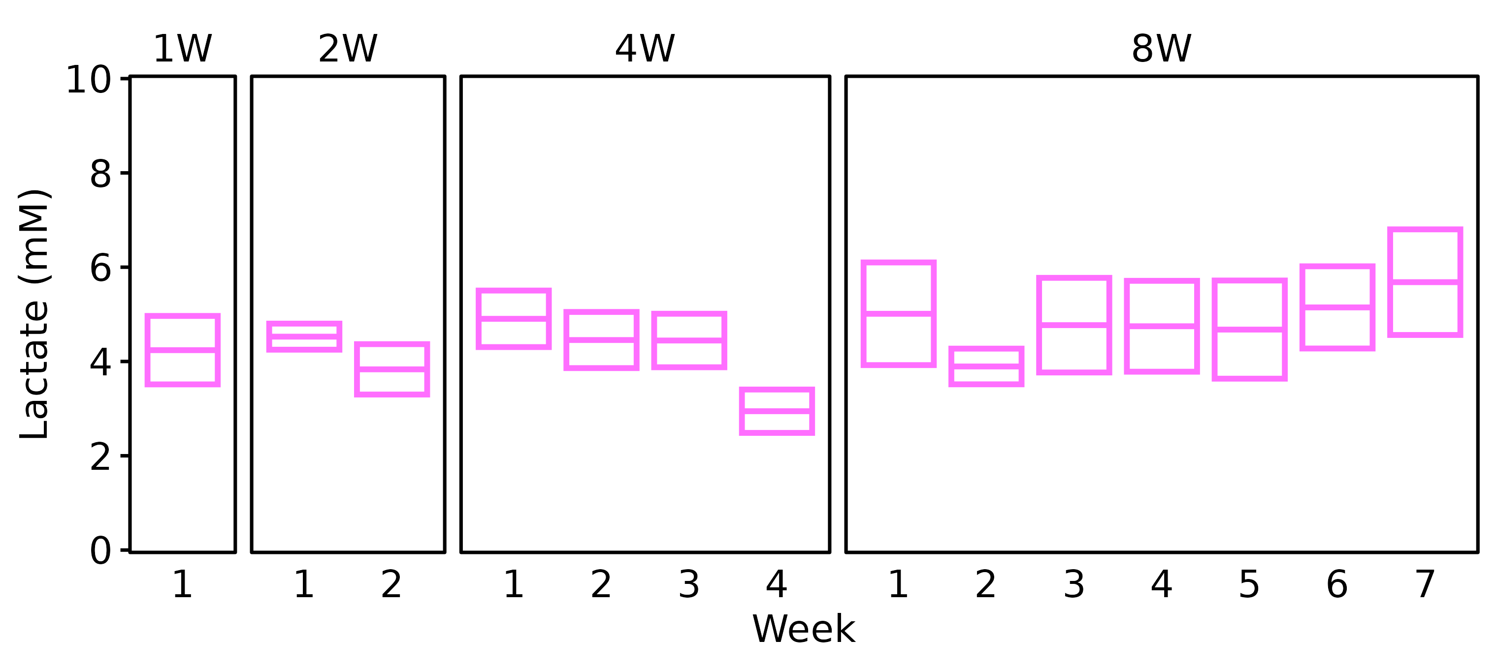
6M Male
# 6M Male
lact_df %>%
  filter(age == "6M", sex == "Male") %>%
  plot_lactate() +
  scale_y_continuous(name = "Lactate (mM)",
                     expand = expansion(mult = 5e-3),
                     breaks = seq(0, 10, 2)) +
  coord_cartesian(ylim = c(0, 10), clip = "off")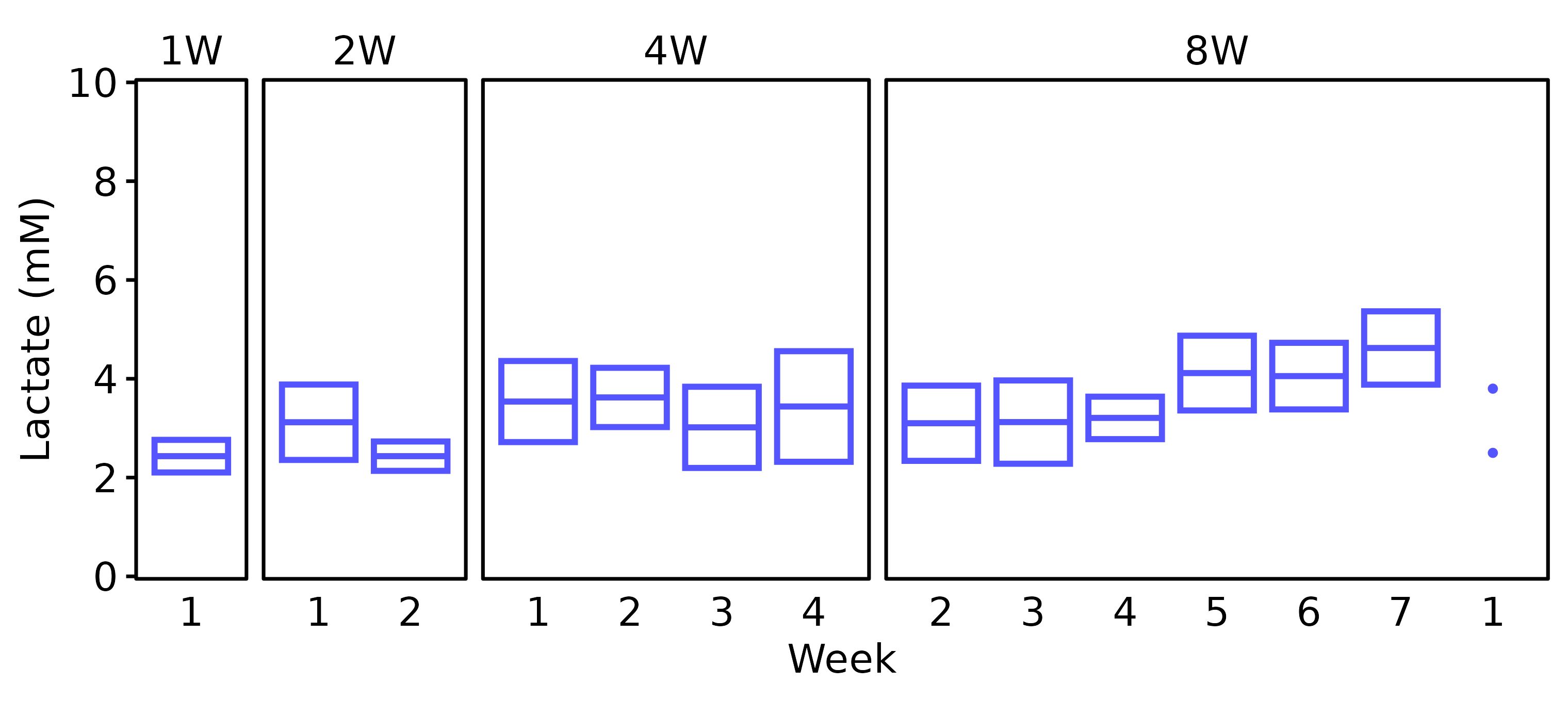
18M Female
# 18M Female
lact_df %>%
  filter(age == "18M", sex == "Female") %>%
  plot_lactate() +
  scale_y_continuous(name = "Lactate (mM)",
                     expand = expansion(mult = 5e-3),
                     breaks = seq(0, 10, 2)) +
  coord_cartesian(ylim = c(0, 10), clip = "off")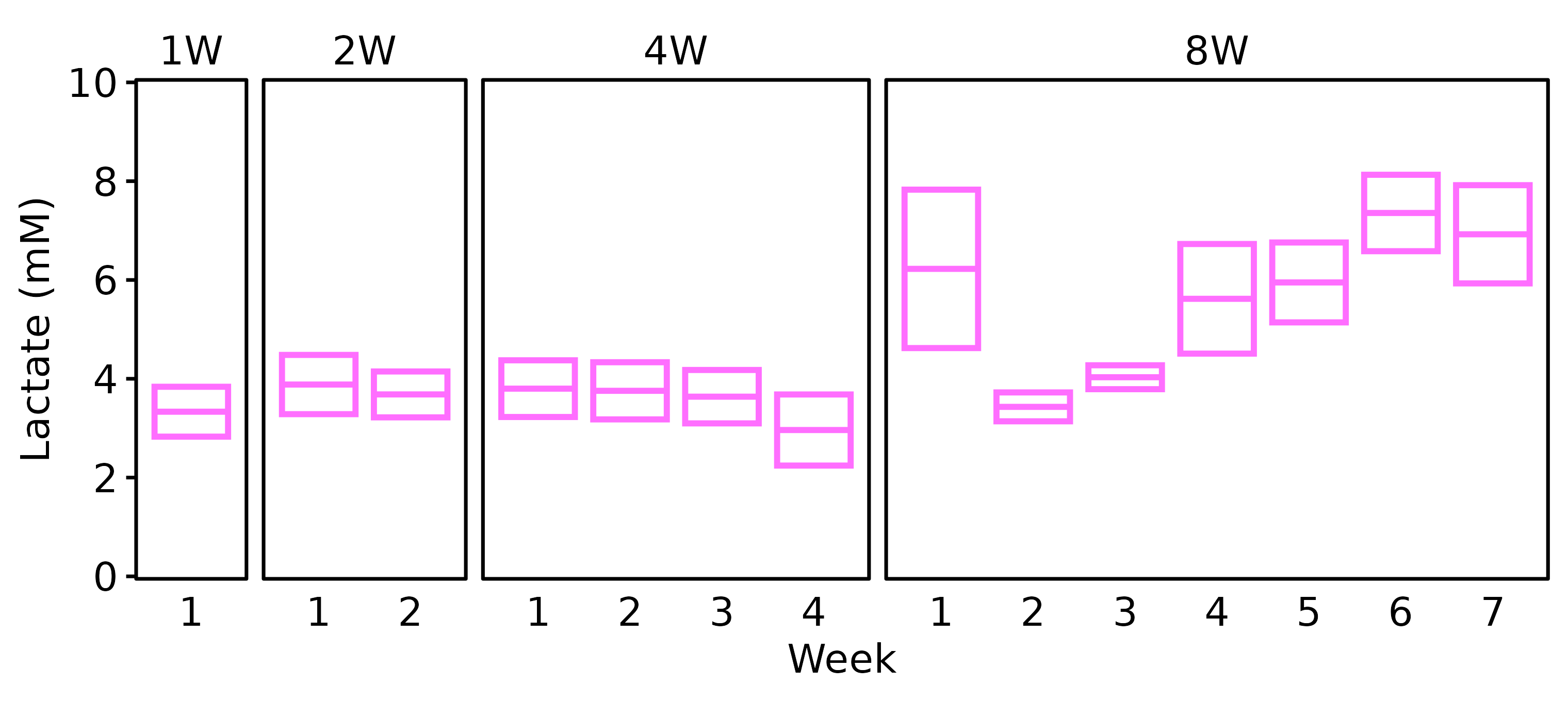
18M Male
# 18M Male
lact_df %>%
  filter(age == "18M", sex == "Male") %>%
  plot_lactate() +
  scale_y_continuous(name = "Lactate (mM)",
                     expand = expansion(mult = 5e-3),
                     breaks = seq(0, 10, 2)) +
  coord_cartesian(ylim = c(0, 10), clip = "off")