Statistical analyses of baseline body composition and VO2max testing measures
Tyler Sagendorf
01 May, 2024
Source:vignettes/BASELINE_STATS.Rmd
BASELINE_STATS.Rmd
# Required packages
library(MotrpacRatTrainingPhysiologyData)
library(ggplot2)
library(MASS)
library(dplyr)
library(emmeans)
library(tibble)
library(tidyr)
library(purrr)
library(latex2exp)
library(rstatix)
theme_set(theme_bw()) # base plot theme
Regression Models
Since all of the measures in this vignette are strictly positive, we will check the mean–variance relationship with code from Dunn and Smyth[1] (pg. 429–430) and fit an appropriate log-link GLM. This allows us to back-transform the means without introducing bias, unlike when the response is transformed. Also, the log-link allows us to test ratios between means, rather than their absolute differences.
Since neither percent fat mass nor percent lean mass approach either of their boundaries of 0 and 100%, we will treat them as if they could take on any positive value. That is, the modeling process will be the same as for the other measures.
If there are obvious problems with the model diagnostic plots, or the mean–variance relationship does not correspond to an exponential family distribution, we will include reciprocal group variances as weights in a log-link Gaussian GLM. Finally, we will remove insignificant predictors to achieve model parsimony based on ANOVA F-tests.
NMR Body Mass
Body mass (g) recorded on the same day as the NMR body composition measures.
# Plot points
ggplot(NMR, aes(x = group, y = pre_body_mass)) +
  geom_point(position = position_jitter(width = 0.15, height = 0)) +
  facet_grid(~ age + sex) +
  theme(axis.text.x = element_text(angle = 90, hjust = 1, vjust = 0.5))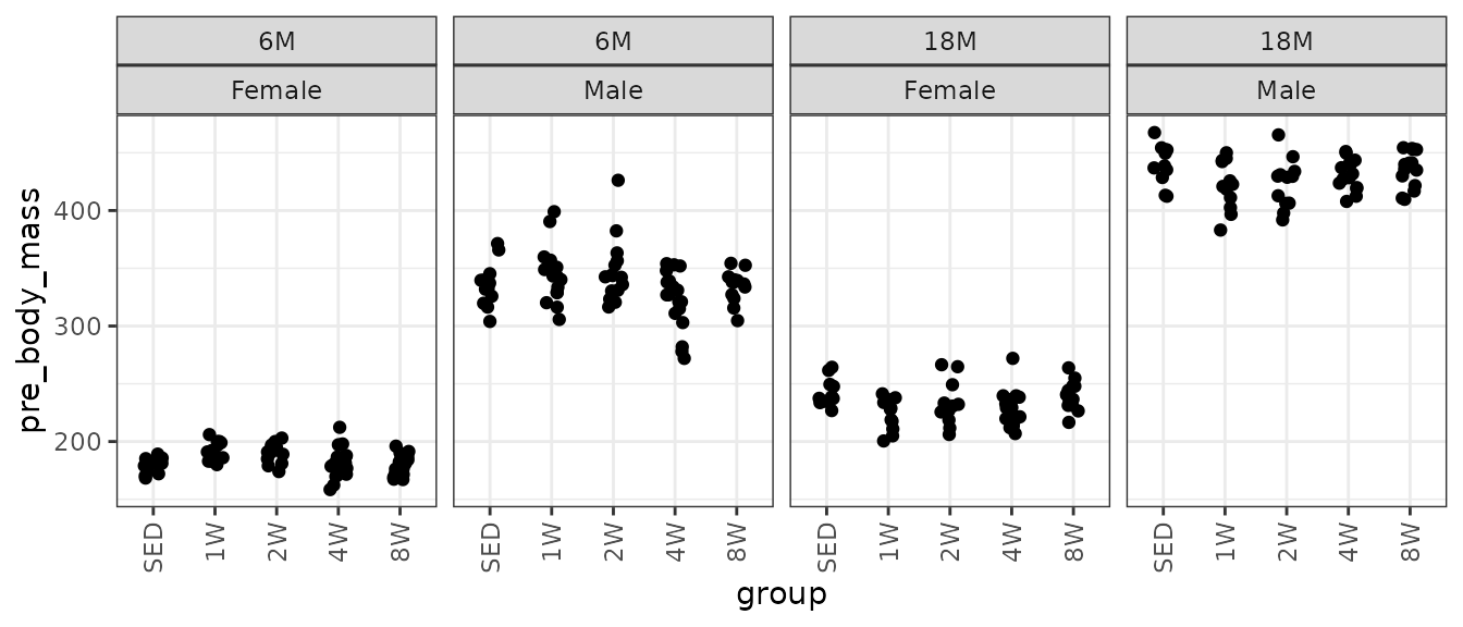
There are no obvious outlying values or other issues. We will check the mean–variance relationship.
mv <- NMR %>%
  group_by(sex, group, age) %>%
  summarise(mn = mean(pre_body_mass),
            vr = var(pre_body_mass))

fit.mv <- lm(log(vr) ~ log(mn), data = mv)
coef(fit.mv)
#> (Intercept)     log(mn)
#>   -4.546389    1.756121
plot(log(vr) ~ log(mn), data = mv, las = 1, pch = 19,
     xlab = "log(group means)", ylab = "log(group variances)")
abline(coef(fit.mv), lwd = 2)
The slope suggests a variance function approximately of the form \(V(\mu) = \mu^{1.76}\). This is close to a gamma distribution, though the plot shows that the relationship is not exactly linear: the variance decreases in the group with the largest mean. Rather than fitting a gamma GLM, we will fit a weighted log-link Gaussian GLM.
wt.body_mass <- NMR %>%
  group_by(age, sex, group) %>%
  mutate(1 / var(pre_body_mass, na.rm = TRUE)) %>%
  pull(-1)

fit.body_mass <- glm(pre_body_mass ~ age * sex * group,
                     family = gaussian("log"),
                     weights = wt.body_mass,
                     data = NMR)
plot_lm(fit.body_mass)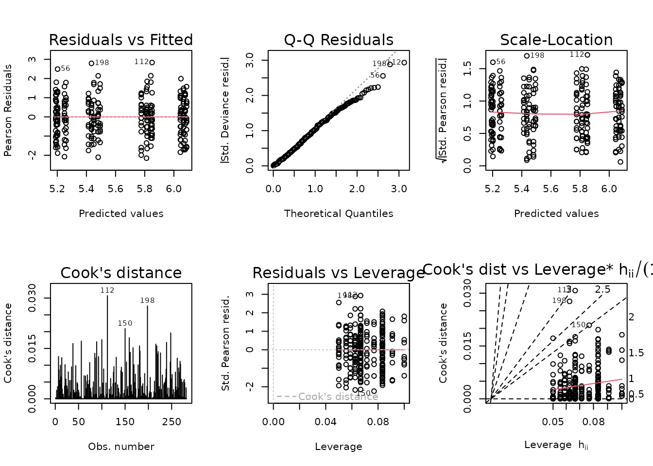
The diagnostic plots seem fine. We will try to simplify the model.
anova(fit.body_mass, test = "F")
#> Analysis of Deviance Table
#>
#> Model: gaussian, link: log
#>
#> Response: pre_body_mass
#>
#> Terms added sequentially (first to last)
#>
#>
#>               Df Deviance Resid. Df Resid. Dev         F    Pr(>F)
#> NULL                            281    13738.7
#> age            1   4596.0       280     9142.7 4596.0140 < 2.2e-16 ***
#> sex            1   8808.7       279      334.1 8808.6692 < 2.2e-16 ***
#> group          4      7.9       275      326.1    1.9840   0.09732 .
#> age:sex        1      1.1       274      325.0    1.1287   0.28903
#> age:group      4     54.4       270      270.6   13.5904 4.412e-10 ***
#> sex:group      4      0.3       266      270.4    0.0645   0.99232
#> age:sex:group  4      8.4       262      262.0    2.0934   0.08204 .
#> ---
#> Signif. codes:  0 '***' 0.001 '**' 0.01 '*' 0.05 '.' 0.1 ' ' 1
fit.body_mass.1 <- update(fit.body_mass, formula = . ~ age * group + sex)
anova(fit.body_mass.1, fit.body_mass, test = "F")
#> Analysis of Deviance Table
#>
#> Model 1: pre_body_mass ~ age + group + sex + age:group
#> Model 2: pre_body_mass ~ age * sex * group
#>   Resid. Df Resid. Dev Df Deviance      F Pr(>F)
#> 1       271     270.73
#> 2       262     262.00  9   8.7277 0.9697 0.4655
There is no significant difference between the models, so we will use the simpler one.
fit.body_mass <- fit.body_mass.1
plot_lm(fit.body_mass)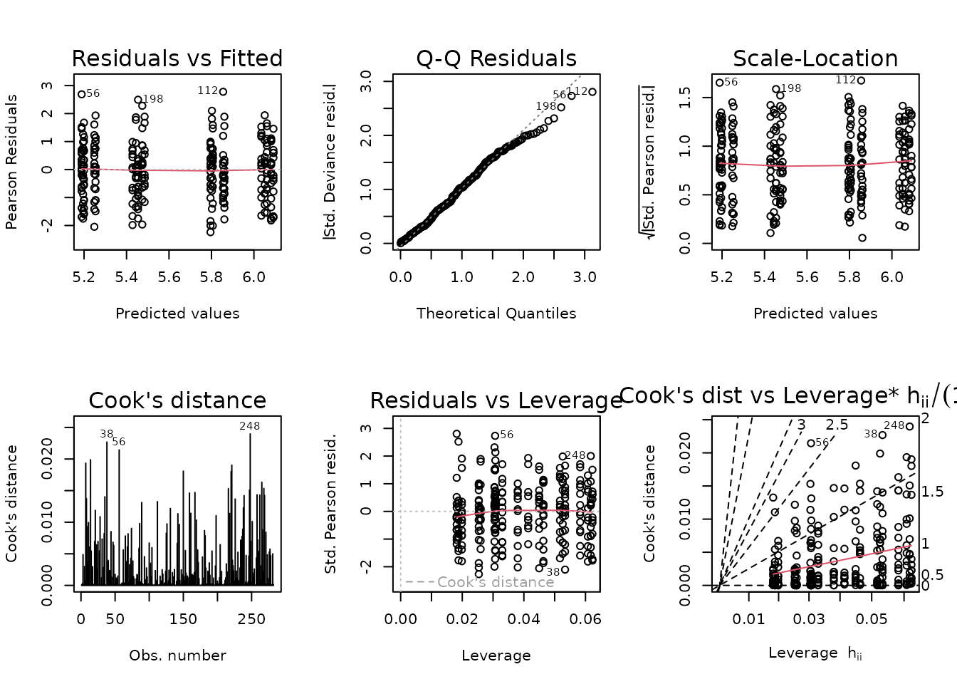
The diagnostic plots still look fine.
summary(fit.body_mass)
#>
#> Call:
#> glm(formula = pre_body_mass ~ age + group + sex + age:group,
#>     family = gaussian("log"), data = NMR, weights = wt.body_mass)
#>
#> Coefficients:
#>                 Estimate Std. Error t value Pr(>|t|)
#> (Intercept)     5.195481   0.009373 554.320  < 2e-16 ***
#> age18M          0.289617   0.013419  21.583  < 2e-16 ***
#> group1W         0.058529   0.012852   4.554 7.96e-06 ***
#> group2W         0.052788   0.013249   3.984 8.70e-05 ***
#> group4W        -0.006799   0.014909  -0.456    0.649
#> group8W         0.004084   0.012411   0.329    0.742
#> sexMale         0.606721   0.006284  96.547  < 2e-16 ***
#> age18M:group1W -0.115395   0.019505  -5.916 9.91e-09 ***
#> age18M:group2W -0.093808   0.020437  -4.590 6.79e-06 ***
#> age18M:group4W -0.024058   0.019202  -1.253    0.211
#> age18M:group8W -0.014997   0.017206  -0.872    0.384
#> ---
#> Signif. codes:  0 '***' 0.001 '**' 0.01 '*' 0.05 '.' 0.1 ' ' 1
#>
#> (Dispersion parameter for gaussian family taken to be 0.9989952)
#>
#>     Null deviance: 13738.74  on 281  degrees of freedom
#> Residual deviance:   270.73  on 271  degrees of freedom
#> AIC: 2320.6
#>
#> Number of Fisher Scoring iterations: 4
NMR Lean Mass
Lean mass (g) recorded via NMR.
# Plot points
ggplot(NMR, aes(x = group, y = pre_lean)) +
  geom_point(position = position_jitter(width = 0.15, height = 0),
             na.rm = TRUE, alpha = 0.5) +
  facet_grid(~ age + sex) +
  theme(axis.text.x = element_text(angle = 90, hjust = 1, vjust = 0.5))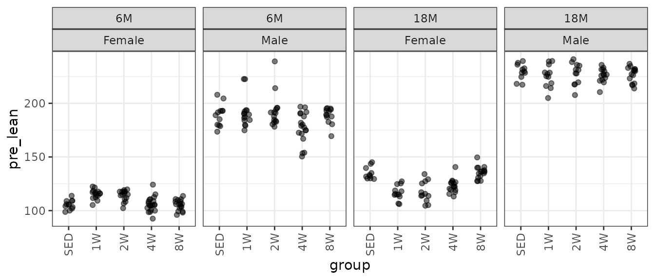
There are several large outlying values in the 6M 1W and 2W male groups. We will check the mean–variance relationship.
mv <- NMR %>%
  group_by(sex, group, age) %>%
  summarise(mn = mean(pre_lean, na.rm = TRUE),
            vr = var(pre_lean, na.rm = TRUE))

fit.mv <- lm(log(vr) ~ log(mn), data = mv)
coef(fit.mv)
#> (Intercept)     log(mn)
#>   -3.582375    1.512023
plot(log(vr) ~ log(mn), data = mv, las = 1, pch = 19,
     xlab = "log(group means)", ylab = "log(group variances)")
abline(coef(fit.mv), lwd = 2)
The slope suggests a variance function approximately of the form \(V(\mu) = \mu^{1.5}\). This is intermediate between the Poisson and gamma distributions, though the plot shows that the relationship is not exactly linear: the variance decreases in the group with the largest mean. Rather than fitting a Poisson or gamma GLM, we will fit a weighted log-link Gaussian GLM.
wt.lean <- NMR %>%
  group_by(age, sex, group) %>%
  mutate(1 / var(pre_lean, na.rm = TRUE)) %>%
  pull(-1)

fit.lean <- glm(pre_lean ~ sex * group * age,
                family = gaussian("log"),
                weights = wt.lean,
                data = NMR)
plot_lm(fit.lean)
The diagnostic plots look fine. We will try to simplify the model.
anova(fit.lean, test = "F")
#> Analysis of Deviance Table
#>
#> Model: gaussian, link: log
#>
#> Response: pre_lean
#>
#> Terms added sequentially (first to last)
#>
#>
#>               Df Deviance Resid. Df Resid. Dev          F    Pr(>F)
#> NULL                            281    12871.5
#> sex            1  11511.5       280     1360.0 11511.5450 < 2.2e-16 ***
#> group          4      1.0       276     1359.0     0.2392  0.915999
#> age            1    924.4       275      434.6   924.4115 < 2.2e-16 ***
#> sex:group      4      6.7       271      427.9     1.6751  0.156105
#> sex:age        1      8.1       270      419.8     8.1378  0.004681 **
#> group:age      4     94.7       266      325.0    23.6824 < 2.2e-16 ***
#> sex:group:age  4     63.0       262      262.0    15.7559  1.44e-11 ***
#> ---
#> Signif. codes:  0 '***' 0.001 '**' 0.01 '*' 0.05 '.' 0.1 ' ' 1
The 3-way interaction is significant, so we will not remove any terms.
summary(fit.lean)
#>
#> Call:
#> glm(formula = pre_lean ~ sex * group * age, family = gaussian("log"),
#>     data = NMR, weights = wt.lean)
#>
#> Coefficients:
#>                          Estimate Std. Error t value Pr(>|t|)
#> (Intercept)             4.6588989  0.0117636 396.044  < 2e-16 ***
#> sexMale                 0.5832307  0.0197269  29.565  < 2e-16 ***
#> group1W                 0.0885367  0.0153876   5.754 2.43e-08 ***
#> group2W                 0.0769667  0.0164390   4.682 4.56e-06 ***
#> group4W                 0.0045687  0.0186064   0.246 0.806227
#> group8W                -0.0031005  0.0164342  -0.189 0.850505
#> age18M                  0.2465072  0.0179188  13.757  < 2e-16 ***
#> sexMale:group1W        -0.0762441  0.0288676  -2.641 0.008759 **
#> sexMale:group2W        -0.0569997  0.0308686  -1.847 0.065944 .
#> sexMale:group4W        -0.0688090  0.0309311  -2.225 0.026961 *
#> sexMale:group8W         0.0004479  0.0253346   0.018 0.985909
#> sexMale:age18M         -0.0528170  0.0257413  -2.052 0.041179 *
#> group1W:age18M         -0.2346420  0.0263665  -8.899  < 2e-16 ***
#> group2W:age18M         -0.2163285  0.0316620  -6.832 5.82e-11 ***
#> group4W:age18M         -0.0961075  0.0263710  -3.644 0.000323 ***
#> group8W:age18M          0.0070771  0.0237770   0.298 0.766209
#> sexMale:group1W:age18M  0.2039115  0.0395161   5.160 4.88e-07 ***
#> sexMale:group2W:age18M  0.1882627  0.0440252   4.276 2.67e-05 ***
#> sexMale:group4W:age18M  0.1453772  0.0381656   3.809 0.000174 ***
#> sexMale:group8W:age18M -0.0159711  0.0330923  -0.483 0.629767
#> ---
#> Signif. codes:  0 '***' 0.001 '**' 0.01 '*' 0.05 '.' 0.1 ' ' 1
#>
#> (Dispersion parameter for gaussian family taken to be 1)
#>
#>     Null deviance: 12872  on 281  degrees of freedom
#> Residual deviance:   262  on 262  degrees of freedom
#> AIC: 1963.6
#>
#> Number of Fisher Scoring iterations: 4
NMR Fat Mass
Fat mass (g) recorded via NMR.
# Plot points
ggplot(NMR, aes(x = group, y = pre_fat)) +
  geom_point(position = position_jitter(width = 0.15, height = 0),
             na.rm = TRUE, alpha = 0.5) +
  facet_grid(~ age + sex) +
  theme(axis.text.x = element_text(angle = 90, hjust = 1, vjust = 0.5))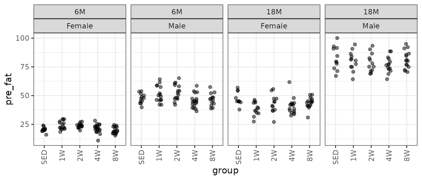
There is one large outlying sample in the 18M 4W female group. We will check the mean–variance relationship.
mv <- NMR %>%
  group_by(sex, group, age) %>%
  summarise(mn = mean(pre_fat, na.rm = TRUE),
            vr = var(pre_fat, na.rm = TRUE))

fit.mv <- lm(log(vr) ~ log(mn), data = mv)
coef(fit.mv)
#> (Intercept)     log(mn)
#>   -2.987518    1.679709
plot(log(vr) ~ log(mn), data = mv, las = 1, pch = 19,
     xlab = "log(group means)", ylab = "log(group variances)")
abline(coef(fit.mv), lwd = 2)
The slope suggests a variance function approximately of the form \(V(\mu) = \mu^{1.68}\), so a gamma GLM may be appropriate.
A few observations appear to be outlying, and the variance seems to decrease slightly at higher expected values. We will try a log-link Gaussian GLM with reciprocal group variance weights instead.
wt.fat <- NMR %>%
group_by(age, sex, group) %>%
mutate(1 / var(pre_fat, na.rm = TRUE)) %>%
pull(-1)
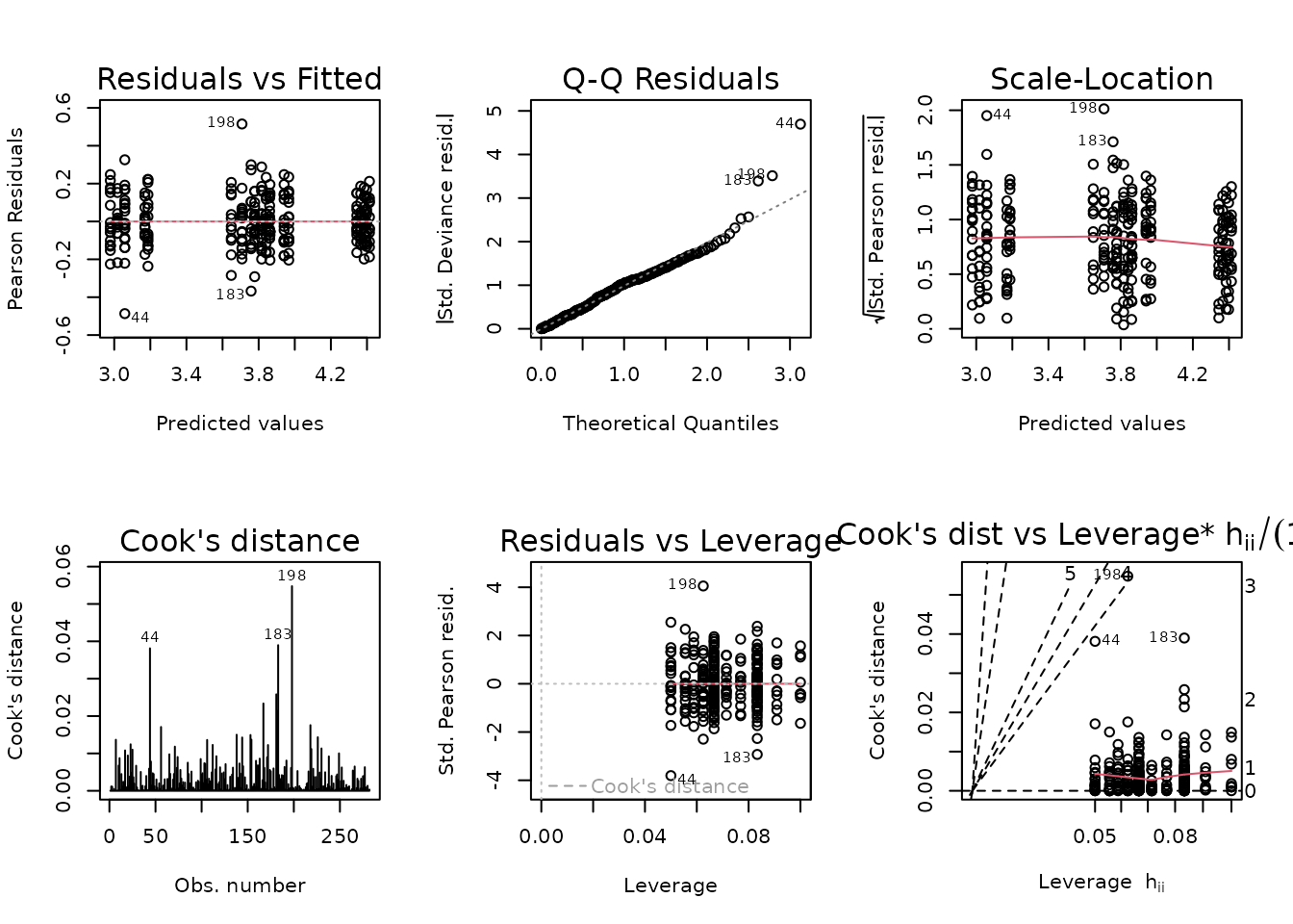
fit.fat <- update(fit.fat, family = gaussian("log"),
weights = wt.fat)
plot_lm(fit.fat)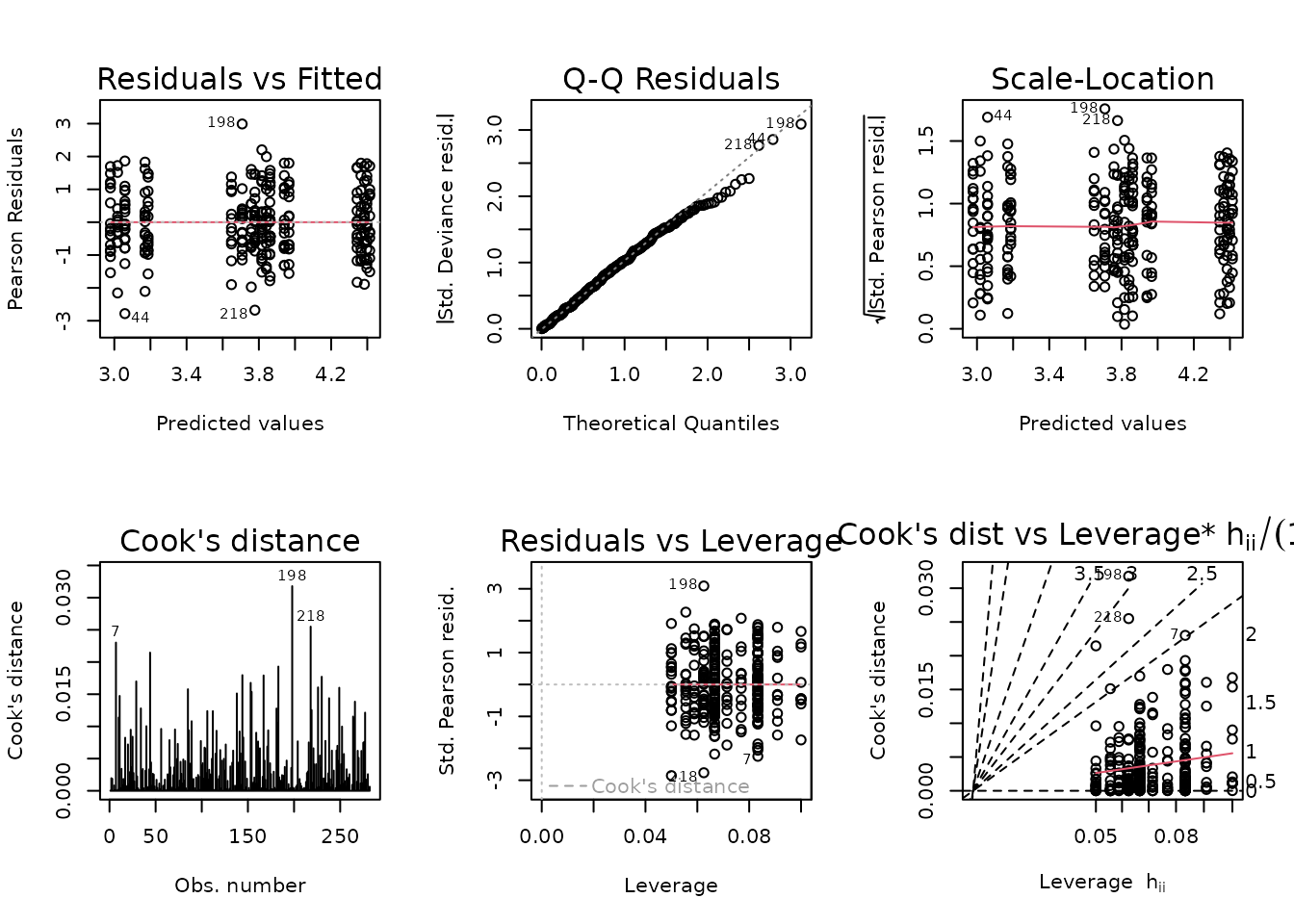
The diagnostic plots look fine. We will try to simplify the model.
anova(fit.fat, test = "F")
#> Analysis of Deviance Table
#>
#> Model: gaussian, link: log
#>
#> Response: pre_fat
#>
#> Terms added sequentially (first to last)
#>
#>
#>               Df Deviance Resid. Df Resid. Dev         F    Pr(>F)
#> NULL                            281     4517.6
#> age            1  2032.33       280     2485.2 2032.3317 < 2.2e-16 ***
#> sex            1  2120.05       279      365.2 2120.0533 < 2.2e-16 ***
#> group          4    15.83       275      349.4    3.9566  0.003896 **
#> age:sex        1    37.15       274      312.2   37.1483 3.897e-09 ***
#> age:group      4    39.47       270      272.7    9.8666 1.888e-07 ***
#> sex:group      4     1.40       266      271.3    0.3488  0.844734
#> age:sex:group  4     9.34       262      262.0    2.3351  0.055996 .
#> ---
#> Signif. codes:  0 '***' 0.001 '**' 0.01 '*' 0.05 '.' 0.1 ' ' 1
We will keep the 3-way interaction, even though it is not significant at the 0.05 level.
summary(fit.fat)
#>
#> Call:
#> glm(formula = pre_fat ~ age + sex + group + age:sex + age:group +
#>     sex:group, family = gaussian("log"), data = NMR, weights = wt.fat)
#>
#> Coefficients:
#>                  Estimate Std. Error t value Pr(>|t|)
#> (Intercept)      3.038185   0.026722 113.696  < 2e-16 ***
#> age18M           0.784785   0.037739  20.795  < 2e-16 ***
#> sexMale          0.805471   0.033735  23.876  < 2e-16 ***
#> group1W          0.100295   0.043321   2.315   0.0214 *
#> group2W          0.132463   0.033390   3.967 9.36e-05 ***
#> group4W          0.000796   0.042374   0.019   0.9850
#> group8W         -0.039416   0.039076  -1.009   0.3140
#> age18M:sexMale  -0.182551   0.030892  -5.909 1.05e-08 ***
#> age18M:group1W  -0.223270   0.049713  -4.491 1.06e-05 ***
#> age18M:group2W  -0.200980   0.049346  -4.073 6.13e-05 ***
#> age18M:group4W  -0.093838   0.047090  -1.993   0.0473 *
#> age18M:group8W  -0.018226   0.045361  -0.402   0.6881
#> sexMale:group1W  0.032614   0.049568   0.658   0.5111
#> sexMale:group2W -0.011028   0.046662  -0.236   0.8134
#> sexMale:group4W -0.016348   0.047962  -0.341   0.7335
#> sexMale:group8W  0.019347   0.044438   0.435   0.6636
#> ---
#> Signif. codes:  0 '***' 0.001 '**' 0.01 '*' 0.05 '.' 0.1 ' ' 1
#>
#> (Dispersion parameter for gaussian family taken to be 1.020081)
#>
#>     Null deviance: 4517.56  on 281  degrees of freedom
#> Residual deviance:  271.34  on 266  degrees of freedom
#> AIC: 1756
#>
#> Number of Fisher Scoring iterations: 4
NMR % Lean Mass
Lean mass (g) recorded via NMR divided by the body mass (g) recorded on the same day and then multiplied by 100%.
# Plot points
ggplot(NMR, aes(x = group, y = pre_lean_pct)) +
  geom_point(position = position_jitter(width = 0.15, height = 0),
             na.rm = TRUE, alpha = 0.5) +
  facet_grid(~ age + sex) +
  theme(axis.text.x = element_text(angle = 90, hjust = 1, vjust = 0.5))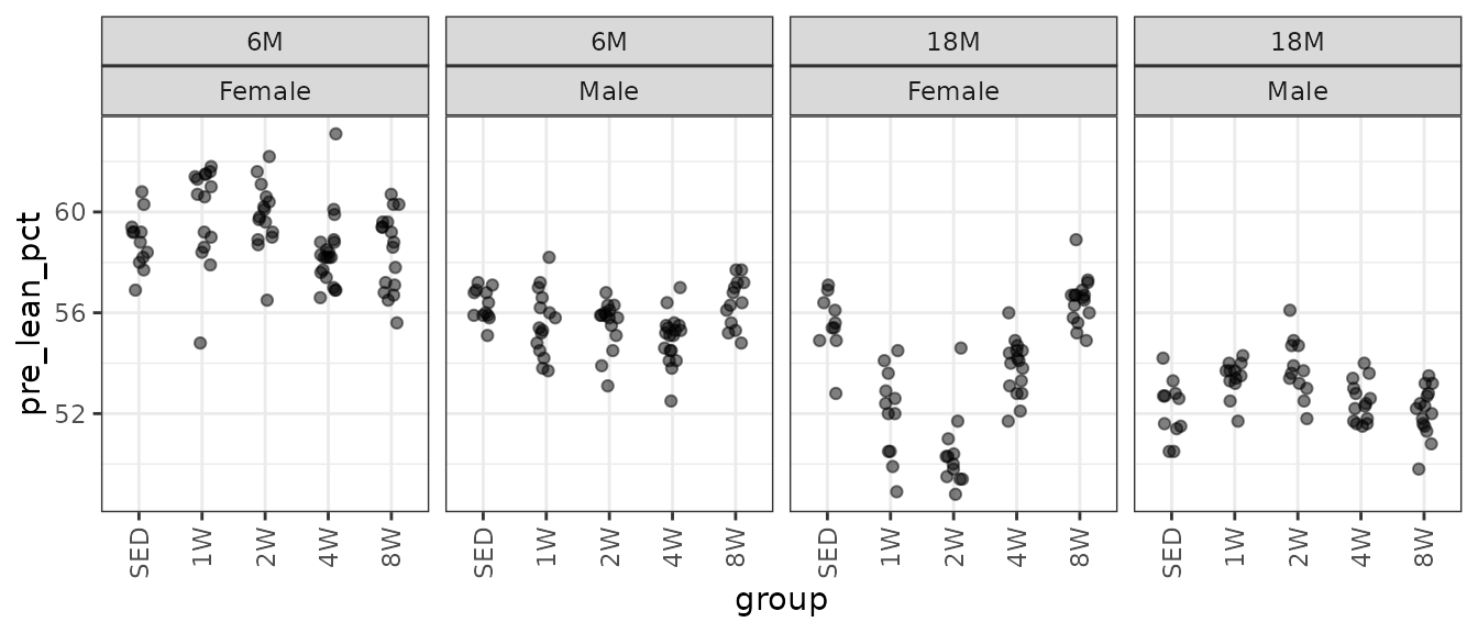
There may be a few outlying values. We will check the mean–variance relationship.
mv <- NMR %>%
  group_by(sex, group, age) %>%
  summarise(mn = mean(pre_lean_pct, na.rm = TRUE),
            vr = var(pre_lean_pct, na.rm = TRUE))

fit.mv <- lm(log(vr) ~ log(mn), data = mv)
coef(fit.mv)
#> (Intercept)     log(mn)
#>   -9.146539    2.344967
plot(log(vr) ~ log(mn), data = mv, las = 1, pch = 19,
     xlab = "log(group means)", ylab = "log(group variances)")
abline(coef(fit.mv), lwd = 2)
The slope suggests a variance function approximately of the form \(V(\mu) = \mu^{2.3}\), so a gamma GLM may be appropriate.
fit.lean_pct <- glm(pre_lean_pct ~ age * sex * group,
                    family = Gamma("log"),
                    data = NMR)
plot_lm(fit.lean_pct)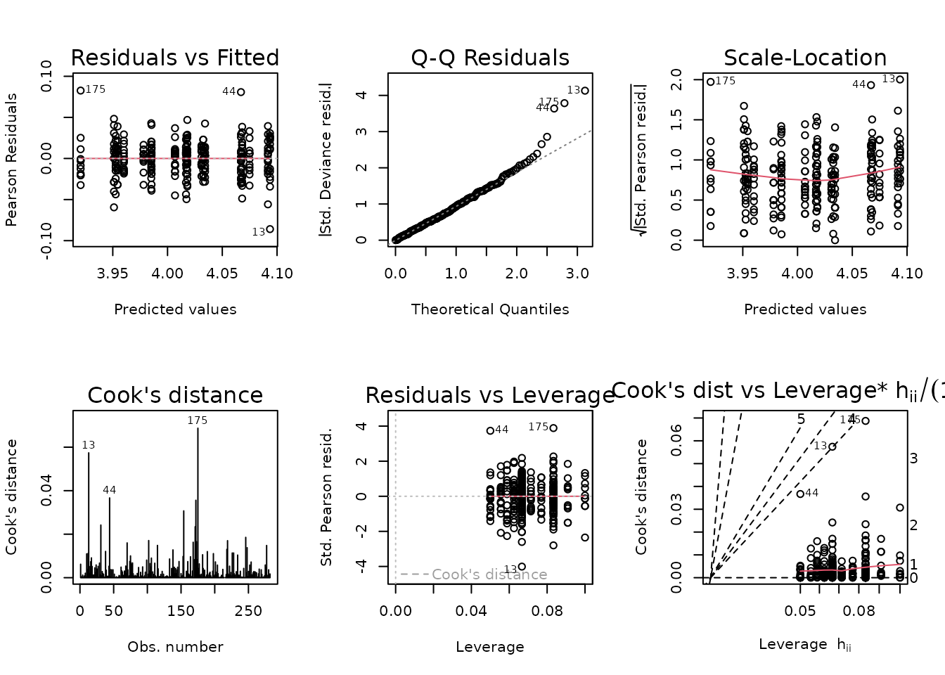
There are a few outliers. We will try a log-link Gaussian GLM with reciprocal group variance weights.
wt.lean_pct <- NMR %>%
  group_by(age, sex, group) %>%
  mutate(1 / var(pre_lean_pct, na.rm = TRUE)) %>%
  pull(-1)

fit.lean_pct <- update(fit.lean_pct,
                       family = gaussian("log"),
                       weights = wt.lean_pct)
plot_lm(fit.lean_pct)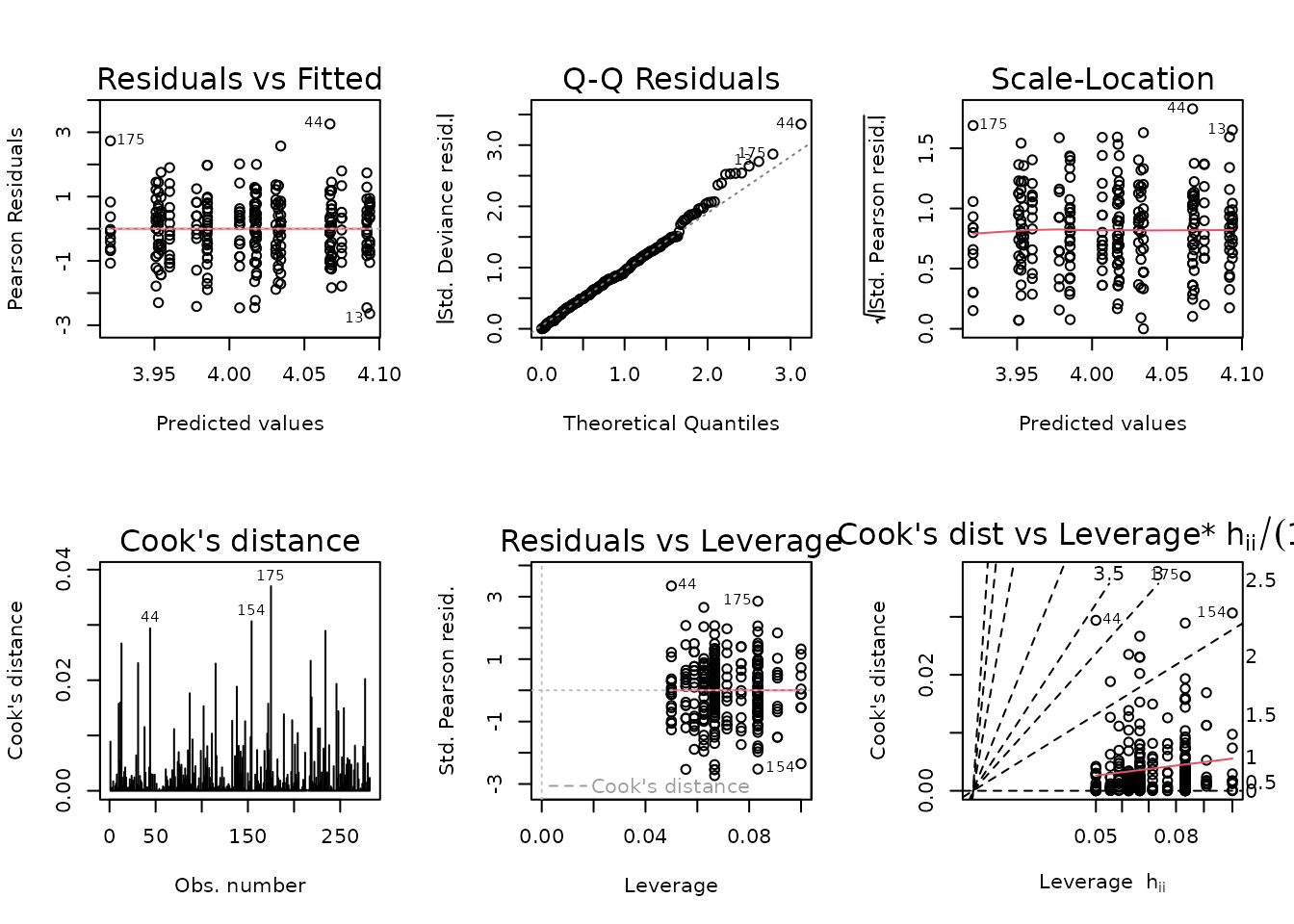
The diagnostic plots look fine now. We will try to simplify the model.
anova(fit.lean_pct, test = "F")
#> Analysis of Deviance Table
#>
#> Model: gaussian, link: log
#>
#> Response: pre_lean_pct
#>
#> Terms added sequentially (first to last)
#>
#>
#>               Df Deviance Resid. Df Resid. Dev        F    Pr(>F)
#> NULL                            281    1584.19
#> age            1   695.35       280     888.84 695.3499 < 2.2e-16 ***
#> sex            1   335.93       279     552.91 335.9266 < 2.2e-16 ***
#> group          4    42.83       275     510.09  10.7066 4.726e-08 ***
#> age:sex        1    23.66       274     486.43  23.6599 1.986e-06 ***
#> age:group      4    15.88       270     470.55   3.9690  0.003816 **
#> sex:group      4    39.54       266     431.01   9.8852 1.831e-07 ***
#> age:sex:group  4   169.01       262     262.00  42.2521 < 2.2e-16 ***
#> ---
#> Signif. codes:  0 '***' 0.001 '**' 0.01 '*' 0.05 '.' 0.1 ' ' 1
All terms are significant, so we will not change the model.
summary(fit.lean_pct)
#>
#> Call:
#> glm(formula = pre_lean_pct ~ age * sex * group, family = gaussian("log"),
#>     data = NMR, weights = wt.lean_pct)
#>
#> Coefficients:
#>                         Estimate Std. Error t value Pr(>|t|)
#> (Intercept)             4.074850   0.005343 762.592  < 2e-16 ***
#> age18M                 -0.057567   0.008826  -6.522 3.55e-10 ***
#> sexMale                -0.043860   0.006284  -6.980 2.42e-11 ***
#> group1W                 0.018716   0.009963   1.879  0.06142 .
#> group2W                 0.016824   0.007935   2.120  0.03492 *
#> group4W                -0.007791   0.007699  -1.012  0.31251
#> group8W                -0.006729   0.008371  -0.804  0.42223
#> age18M:sexMale         -0.019038   0.011571  -1.645  0.10110
#> age18M:group1W         -0.084916   0.015534  -5.467 1.07e-07 ***
#> age18M:group2W         -0.113455   0.013730  -8.263 7.12e-15 ***
#> age18M:group4W         -0.024103   0.011632  -2.072  0.03923 *
#> age18M:group8W          0.023686   0.011682   2.028  0.04362 *
#> sexMale:group1W        -0.031643   0.012118  -2.611  0.00954 **
#> sexMale:group2W        -0.030951   0.009750  -3.174  0.00168 **
#> sexMale:group4W        -0.016371   0.009423  -1.737  0.08349 .
#> sexMale:group8W         0.008344   0.010170   0.820  0.41271
#> age18M:sexMale:group1W  0.121581   0.018673   6.511 3.79e-10 ***
#> age18M:sexMale:group2W  0.158315   0.017465   9.065  < 2e-16 ***
#> age18M:sexMale:group4W  0.054012   0.015060   3.586  0.00040 ***
#> age18M:sexMale:group8W -0.027034   0.015457  -1.749  0.08147 .
#> ---
#> Signif. codes:  0 '***' 0.001 '**' 0.01 '*' 0.05 '.' 0.1 ' ' 1
#>
#> (Dispersion parameter for gaussian family taken to be 1.000001)
#>
#>     Null deviance: 1584.2  on 281  degrees of freedom
#> Residual deviance:  262.0  on 262  degrees of freedom
#> AIC: 900.2
#>
#> Number of Fisher Scoring iterations: 3
NMR % Fat Mass
Fat mass (g) recorded via NMR divided by the body mass (g) recorded on the same day and then multiplied by 100%.
# Plot points
ggplot(NMR, aes(x = group, y = pre_fat_pct)) +
  geom_point(position = position_jitter(width = 0.15, height = 0),
             na.rm = TRUE, alpha = 0.5) +
  facet_grid(~ age + sex) +
  theme(axis.text.x = element_text(angle = 90, hjust = 1, vjust = 0.5))
There may be a few outlying values. We will check the mean–variance relationship.
mv <- NMR %>%
  group_by(sex, group, age) %>%
  summarise(mn = mean(pre_fat_pct, na.rm = TRUE),
            vr = var(pre_fat_pct, na.rm = TRUE))

fit.mv <- lm(log(vr) ~ log(mn), data = mv)
coef(fit.mv)
#> (Intercept)     log(mn)
#>   -2.815588    1.277487
plot(log(vr) ~ log(mn), data = mv, las = 1, pch = 19,
     xlab = "log(group means)", ylab = "log(group variances)")
abline(coef(fit.mv), lwd = 2)
The slope suggests a variance function approximately of the form \(V(\mu) = \mu^{1.3}\), so a quasi-Poisson GLM may be appropriate.
fit.fat_pct <- glm(pre_fat_pct ~ age * sex * group,
                   family = quasipoisson("log"),
                   data = NMR)
plot_lm(fit.fat_pct)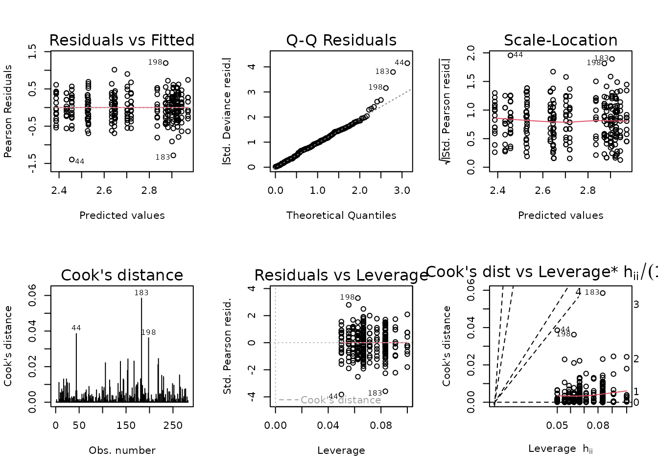
The diagnostic plots seem fine. We will try to simplify the model.
anova(fit.fat_pct, test = "F")
#> Analysis of Deviance Table
#>
#> Model: quasipoisson, link: log
#>
#> Response: pre_fat_pct
#>
#> Terms added sequentially (first to last)
#>
#>
#>               Df Deviance Resid. Df Resid. Dev        F    Pr(>F)
#> NULL                            281    187.982
#> age            1  123.253       280     64.729 881.6948 < 2.2e-16 ***
#> sex            1   12.379       279     52.350  88.5499 < 2.2e-16 ***
#> group          4    1.985       275     50.365   3.5504 0.0076799 **
#> age:sex        1    8.674       274     41.691  62.0479  8.96e-14 ***
#> age:group      4    3.106       270     38.585   5.5550 0.0002627 ***
#> sex:group      4    0.491       266     38.094   0.8786 0.4772209
#> age:sex:group  4    1.053       262     37.041   1.8829 0.1137809
#> ---
#> Signif. codes:  0 '***' 0.001 '**' 0.01 '*' 0.05 '.' 0.1 ' ' 1
fit.fat_pct.1 <- update(fit.fat_pct, formula = . ~ age * (sex + group))
anova(fit.fat_pct.1, fit.fat_pct, test = "F")
#> Analysis of Deviance Table
#>
#> Model 1: pre_fat_pct ~ age + sex + group + age:sex + age:group
#> Model 2: pre_fat_pct ~ age * sex * group
#>   Resid. Df Resid. Dev Df Deviance      F Pr(>F)
#> 1       270     38.585
#> 2       262     37.041  8   1.5441 1.3807  0.205
There is no significant difference between the models, so we will use the simpler one.
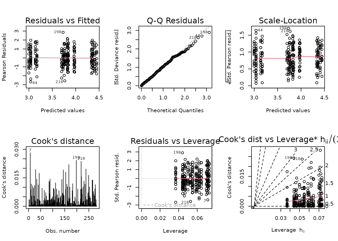
fit.fat_pct <- fit.fat_pct.1
plot_lm(fit.fat_pct)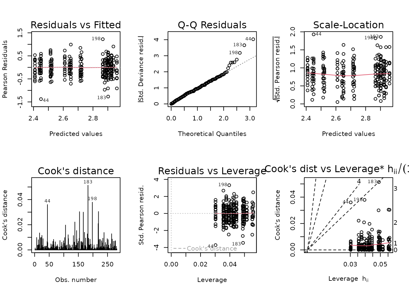
summary(fit.fat_pct)
#>
#> Call:
#> glm(formula = pre_fat_pct ~ age + sex + group + age:sex + age:group,
#>     family = quasipoisson("log"), data = NMR)
#>
#> Coefficients:
#>                 Estimate Std. Error t value Pr(>|t|)
#> (Intercept)     2.440973   0.023410 104.271  < 2e-16 ***
#> age18M          0.496418   0.031098  15.963  < 2e-16 ***
#> sexMale         0.200994   0.016924  11.877  < 2e-16 ***
#> group1W         0.073557   0.028360   2.594  0.01001 *
#> group2W         0.081052   0.028314   2.863  0.00453 **
#> group4W         0.009247   0.027419   0.337  0.73619
#> group8W        -0.031631   0.029133  -1.086  0.27857
#> age18M:sexMale -0.177647   0.022899  -7.758 1.78e-13 ***
#> age18M:group1W -0.132087   0.038520  -3.429  0.00070 ***
#> age18M:group2W -0.116476   0.038389  -3.034  0.00265 **
#> age18M:group4W -0.080465   0.037014  -2.174  0.03058 *
#> age18M:group8W -0.004775   0.038068  -0.125  0.90028
#> ---
#> Signif. codes:  0 '***' 0.001 '**' 0.01 '*' 0.05 '.' 0.1 ' ' 1
#>
#> (Dispersion parameter for quasipoisson family taken to be 0.1413136)
#>
#>     Null deviance: 187.982  on 281  degrees of freedom
#> Residual deviance:  38.585  on 270  degrees of freedom
#> AIC: NA
#>
#> Number of Fisher Scoring iterations: 4
Absolute VO\(_2\)max
Absolute VO\(_2\)max is calculated by multiplying relative VO\(_2\)max (\(mL \cdot kg^{-1} \cdot min^{-1}\)) by body mass (kg).
# Plot points
ggplot(VO2MAX, aes(x = group, y = pre_vo2max_ml_min)) +
  geom_point(position = position_jitter(width = 0.15, height = 0),
             na.rm = TRUE, alpha = 0.5) +
  facet_grid(~ age + sex) +
  theme(axis.text.x = element_text(angle = 90, hjust = 1, vjust = 0.5))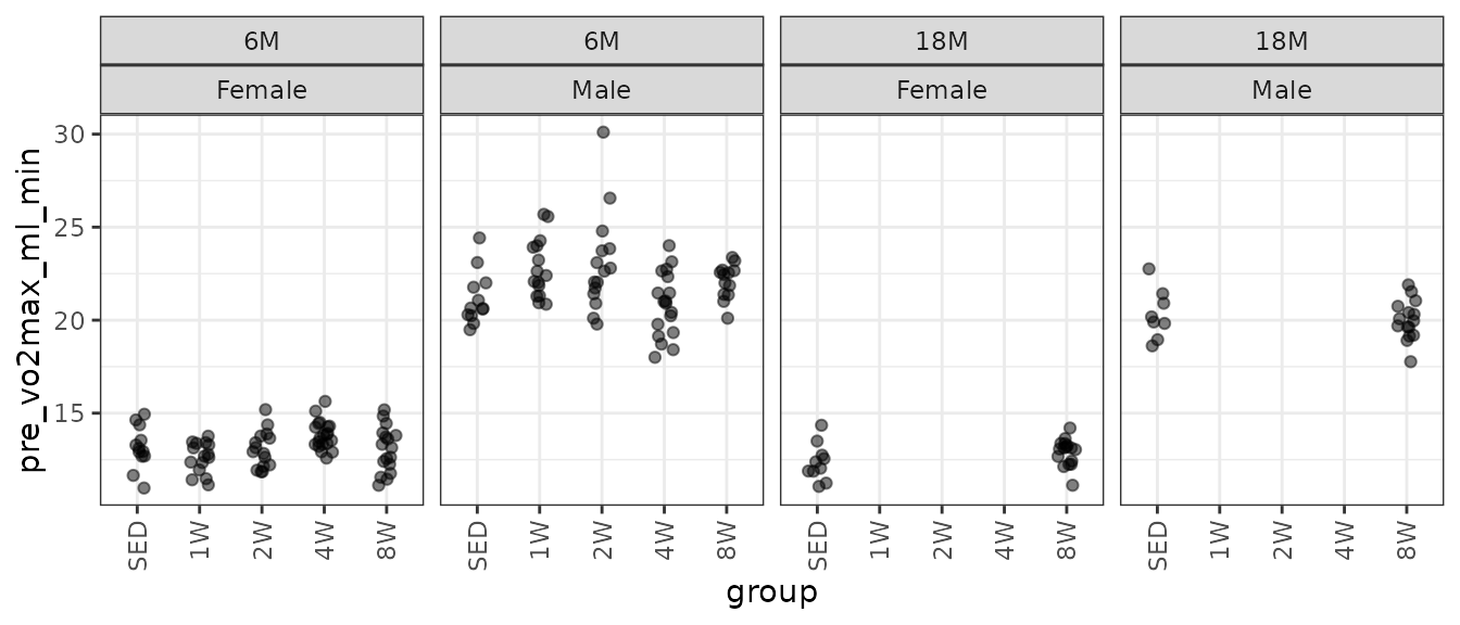
There is a large outlying value in the 6M 2W male group. It is the largest value overall.
filter(VO2MAX, age == "6M") %>%
  ggplot(aes(x = pre_body_mass, y = pre_vo2max_ml_min)) +
  geom_point(na.rm = TRUE, alpha = 0.5)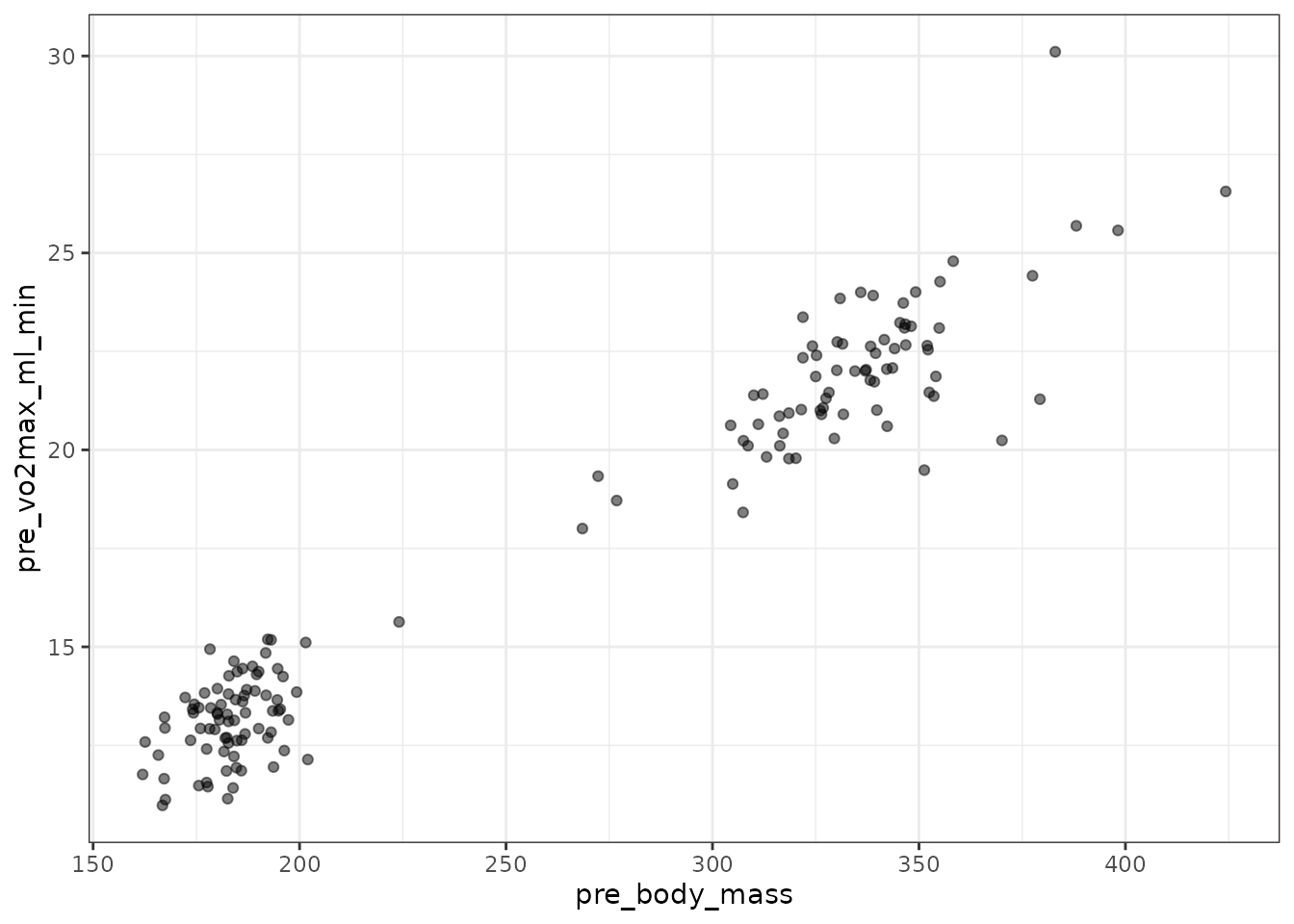
That outlier has one of the highest body masses, though it is not unusual. We will determine the mean–variance relationship.
mv <- VO2MAX %>%
  group_by(age, sex, group) %>%
  summarise(mn = mean(pre_vo2max_ml_min, na.rm = TRUE),
            vr = var(pre_vo2max_ml_min, na.rm = TRUE))

fit.mv <- lm(log(vr) ~ log(mn), data = mv)
coef(fit.mv)
#> (Intercept)     log(mn)
#>   -4.793618    1.812129
plot(log(vr) ~ log(mn), data = mv, las = 1, pch = 19,
     xlab = "log(group means)", ylab = "log(group variances)")
abline(coef(fit.mv), lwd = 2)
The slope suggests a variance function approximately of the form \(V(\mu) = \mu^{1.5}\). This is intermediate between the Poisson and gamma distributions. We will fit a log-link gamma GLM. We will need to combine age and group or some coefficients will be inestimable. Note that the point with the largest variance on the plot is the group with that outlier.
# Concatenate age and group
VO2MAX <- mutate(VO2MAX, age_group = paste0(age, "_", group))

fit.vo2max_abs <- glm(pre_vo2max_ml_min ~ age_group * sex,
                      family = Gamma("log"),
                      data = VO2MAX)
plot_lm(fit.vo2max_abs)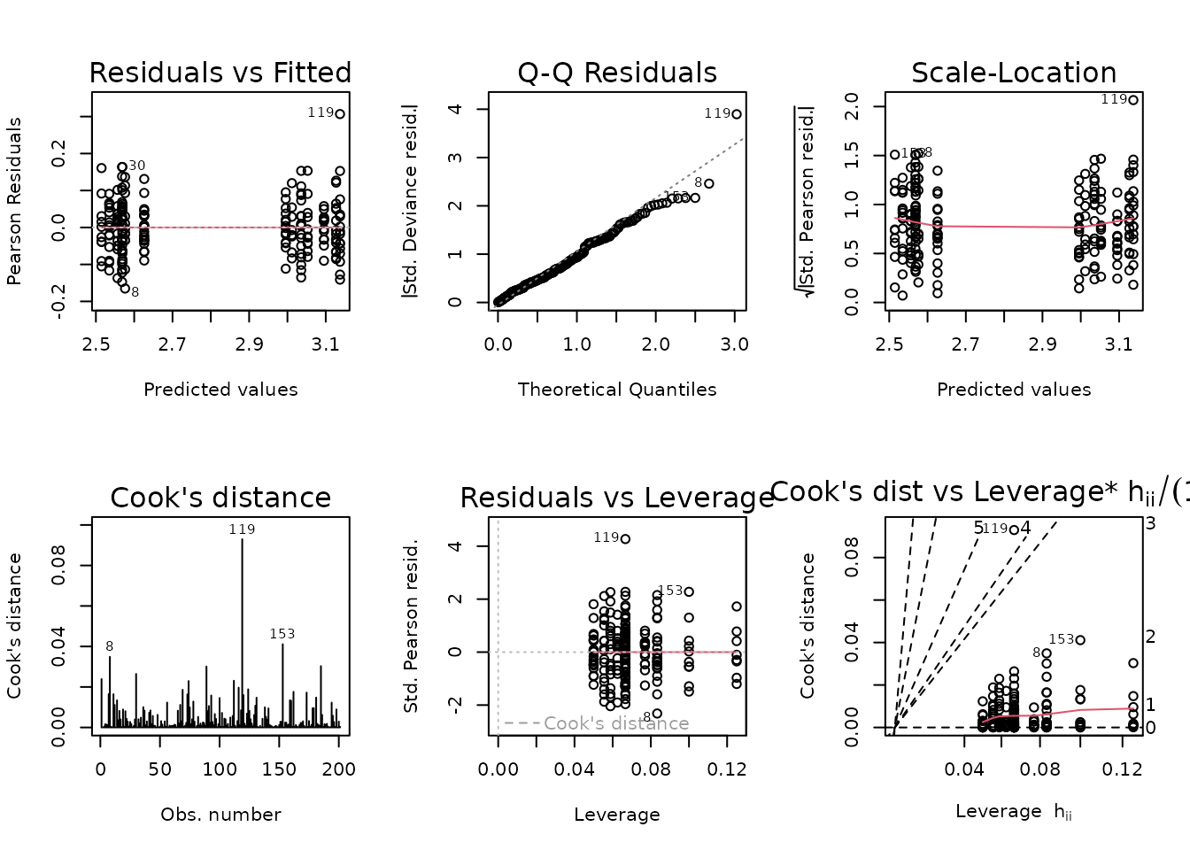
Observation 119 has a large residual, but does not appear to substantially affect the fit. However, removal will bring the mean of that group closer to its matching SED group, so the results of that comparison will be more conservative. This is the approach we will take.
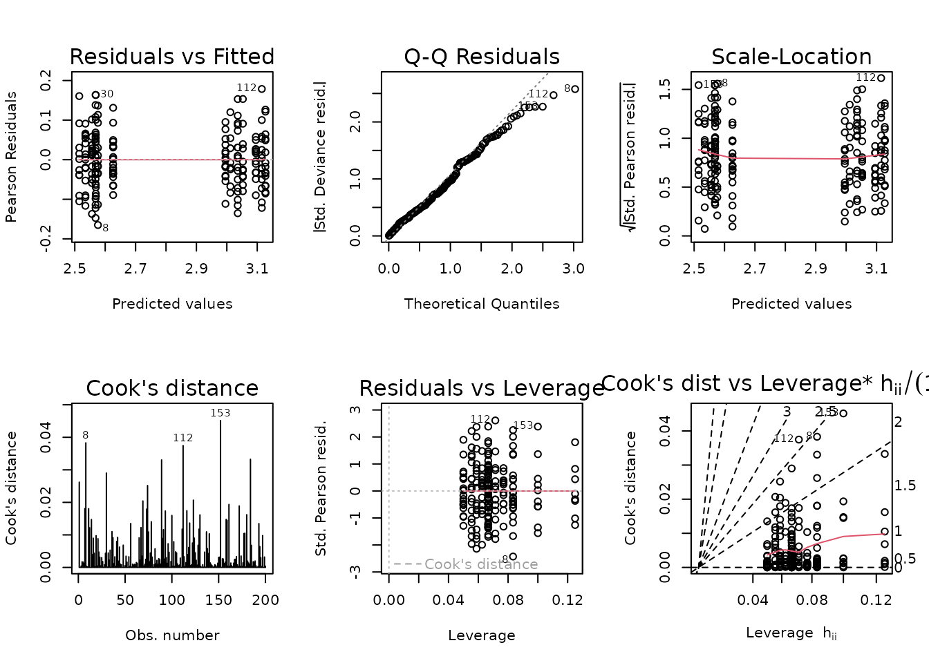
The diagnostic plots look fine now, so we will try to simplify the model.
anova(fit.vo2max_abs, test = "F")
#> Analysis of Deviance Table
#>
#> Model: Gamma, link: log
#>
#> Response: pre_vo2max_ml_min
#>
#> Terms added sequentially (first to last)
#>
#>
#>               Df Deviance Resid. Df Resid. Dev         F    Pr(>F)
#> NULL                            199    13.4977
#> age_group      6   0.2221       193    13.2755    7.3426 4.649e-07 ***
#> sex            1  12.1497       192     1.1258 2409.5125 < 2.2e-16 ***
#> age_group:sex  6   0.1918       186     0.9340    6.3406 4.351e-06 ***
#> ---
#> Signif. codes:  0 '***' 0.001 '**' 0.01 '*' 0.05 '.' 0.1 ' ' 1
All terms are significant.
summary(fit.vo2max_abs)
#>
#> Call:
#> glm(formula = pre_vo2max_ml_min ~ age_group * sex, family = Gamma("log"),
#>     data = VO2MAX, subset = -119)
#>
#> Coefficients:
#>                          Estimate Std. Error t value Pr(>|t|)
#> (Intercept)               2.55648    0.01775 144.007  < 2e-16 ***
#> age_group18M_SED         -0.04175    0.02862  -1.458  0.14642
#> age_group6M_1W           -0.02156    0.02552  -0.845  0.39940
#> age_group6M_2W            0.01264    0.02552   0.495  0.62099
#> age_group6M_4W            0.06964    0.02382   2.924  0.00388 **
#> age_group6M_8W            0.01186    0.02473   0.480  0.63207
#> age_group6M_SED           0.01964    0.02712   0.724  0.46982
#> sexMale                   0.43907    0.02552  17.205  < 2e-16 ***
#> age_group18M_SED:sexMale  0.05780    0.04226   1.368  0.17307
#> age_group6M_1W:sexMale    0.15295    0.03638   4.204 4.07e-05 ***
#> age_group6M_2W:sexMale    0.10685    0.03671   2.911  0.00405 **
#> age_group6M_4W:sexMale   -0.02931    0.03440  -0.852  0.39530
#> age_group6M_8W:sexMale    0.08787    0.03655   2.404  0.01719 *
#> age_group6M_SED:sexMale   0.03754    0.03862   0.972  0.33237
#> ---
#> Signif. codes:  0 '***' 0.001 '**' 0.01 '*' 0.05 '.' 0.1 ' ' 1
#>
#> (Dispersion parameter for Gamma family taken to be 0.005042403)
#>
#>     Null deviance: 13.49768  on 199  degrees of freedom
#> Residual deviance:  0.93397  on 186  degrees of freedom
#>   (33 observations deleted due to missingness)
#> AIC: 645.01
#>
#> Number of Fisher Scoring iterations: 3
Relative VO\(_2\)max
Relative VO\(_2\)max (mL/kg body mass/min).
# Plot points
ggplot(VO2MAX, aes(x = group, y = pre_vo2max_ml_kg_min)) +
  geom_point(position = position_jitter(width = 0.15, height = 0),
             na.rm = TRUE, alpha = 0.5) +
  facet_grid(~ age + sex) +
  theme(axis.text.x = element_text(angle = 90, hjust = 1, vjust = 0.5))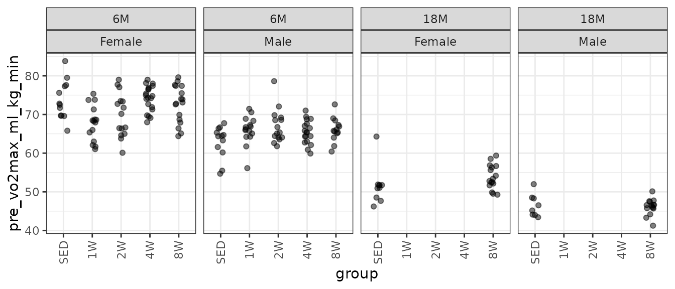
There is an extreme observation in the 18M SED female group. We will check the mean–variance relationship.
mv <- VO2MAX %>%
  group_by(age, sex, group) %>%
  summarise(mn = mean(pre_vo2max_ml_min, na.rm = TRUE),
            vr = var(pre_vo2max_ml_min, na.rm = TRUE))

fit.mv <- lm(log(vr) ~ log(mn), data = mv)
coef(fit.mv)
#> (Intercept)     log(mn)
#>   -4.793618    1.812129
plot(log(vr) ~ log(mn), data = mv, las = 1, pch = 19,
     xlab = "log(group means)", ylab = "log(group variances)")
abline(coef(fit.mv), lwd = 2)
The slope suggests a variance function approximately of the form \(V(\mu) = \mu^{1.5}\). This is intermediate between the Poisson and gamma distributions. We will fit a log-link gamma GLM.
fit.vo2max_rel <- glm(pre_vo2max_ml_kg_min ~ age_group * sex,
                      family = Gamma("log"),
                      data = VO2MAX)
plot_lm(fit.vo2max_rel)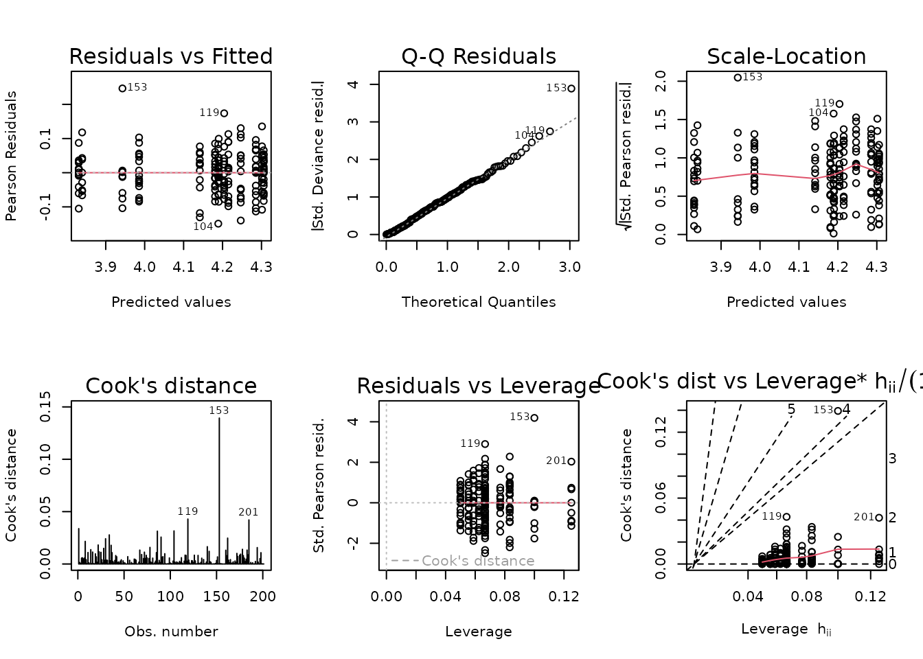
Observation 153 has a large residual, but does not substantially affect the model fit. Removal will bring the mean of that group closer to the rest, however, so we will do so. This ensures the comparison against the SED group will produce more conservative results.
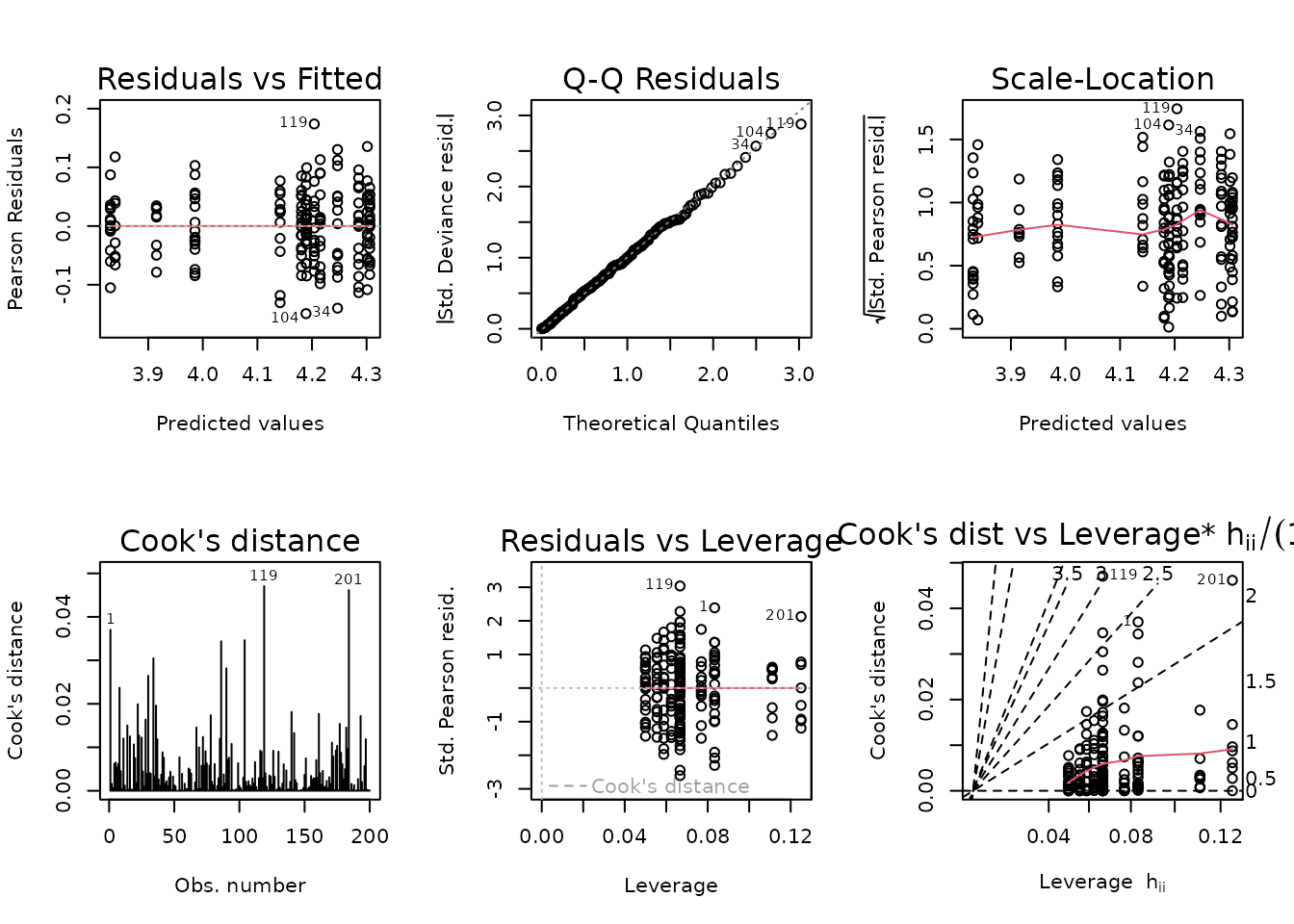
The diagnostic plots look fine, so we will try to simplify the model.
anova(fit.vo2max_rel, test = "F")
#> Analysis of Deviance Table
#>
#> Model: Gamma, link: log
#>
#> Response: pre_vo2max_ml_kg_min
#>
#> Terms added sequentially (first to last)
#>
#>
#>               Df Deviance Resid. Df Resid. Dev        F    Pr(>F)
#> NULL                            199     5.0222
#> age_group      6   3.7708       193     1.2514 178.9303 < 2.2e-16 ***
#> sex            1   0.4763       192     0.7751 135.6037 < 2.2e-16 ***
#> age_group:sex  6   0.1189       186     0.6562   5.6428 2.095e-05 ***
#> ---
#> Signif. codes:  0 '***' 0.001 '**' 0.01 '*' 0.05 '.' 0.1 ' ' 1
All terms are significant.
summary(fit.vo2max_rel)
#>
#> Call:
#> glm(formula = pre_vo2max_ml_kg_min ~ age_group * sex, family = Gamma("log"),
#>     data = VO2MAX, subset = -153)
#>
#> Coefficients:
#>                           Estimate Std. Error t value Pr(>|t|)
#> (Intercept)               3.985622   0.014816 269.001  < 2e-16 ***
#> age_group18M_SED         -0.070515   0.024694  -2.856 0.004785 **
#> age_group6M_1W            0.229356   0.021300  10.768  < 2e-16 ***
#> age_group6M_2W            0.261158   0.021300  12.261  < 2e-16 ***
#> age_group6M_4W            0.320111   0.019878  16.104  < 2e-16 ***
#> age_group6M_8W            0.299910   0.020643  14.528  < 2e-16 ***
#> age_group6M_SED           0.315737   0.022632  13.951  < 2e-16 ***
#> sexMale                  -0.154896   0.021300  -7.272 9.54e-12 ***
#> age_group18M_SED:sexMale  0.079187   0.035819   2.211 0.028272 *
#> age_group6M_1W:sexMale    0.128976   0.030365   4.248 3.41e-05 ***
#> age_group6M_2W:sexMale    0.112291   0.030365   3.698 0.000286 ***
#> age_group6M_4W:sexMale    0.029949   0.028713   1.043 0.298286
#> age_group6M_8W:sexMale    0.059566   0.030504   1.953 0.052350 .
#> age_group6M_SED:sexMale  -0.004851   0.032235  -0.150 0.880552
#> ---
#> Signif. codes:  0 '***' 0.001 '**' 0.01 '*' 0.05 '.' 0.1 ' ' 1
#>
#> (Dispersion parameter for Gamma family taken to be 0.003512395)
#>
#>     Null deviance: 5.02221  on 199  degrees of freedom
#> Residual deviance: 0.65616  on 186  degrees of freedom
#>   (33 observations deleted due to missingness)
#> AIC: 1113.1
#>
#> Number of Fisher Scoring iterations: 3
Maximum Run Speed
Since run speed was increased in 1.8 m/min increments, as defined in the training protocol, it may be preferable to use a non-parametric test. Rather than plotting the individual points, since they can only take on a few different values, we will instead count the number of samples that take on a particular value in each group and scale the points accordingly.
# Plot points
VO2MAX %>%
  count(age, sex, group, pre_speed_max) %>%
  ggplot(aes(x = group, y = pre_speed_max, size = n)) +
  geom_point(na.rm = TRUE) +
  facet_grid(~ age + sex) +
  scale_size_area(max_size = 5) +
  theme(axis.text.x = element_text(angle = 90, hjust = 1, vjust = 0.5))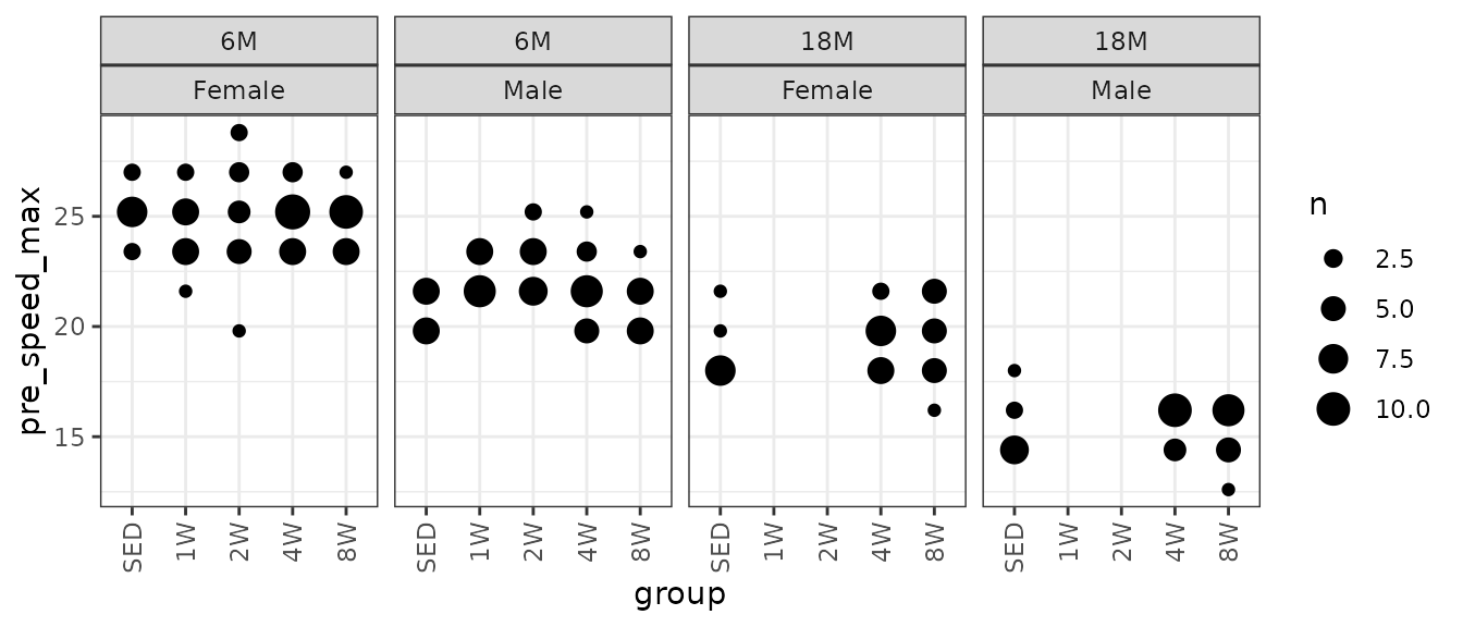
We will use Wilcoxon Rank Sum tests to compare each trained group to their matching control group. We will adjust p-values within each age and sex group after we set up comparisons for all measures.
# Testing the differences is equivalent to a paired test
speed_res <- VO2MAX %>%
  group_by(age, sex) %>%
  wilcox_test(formula = pre_speed_max ~ group, mu = 0,
              detailed = TRUE, ref.group = "SED",
              p.adjust.method = "none") %>%
  as.data.frame() %>%
  # Rename columns to match emmeans output
  dplyr::rename(p.value = p,
                lower.CL = conf.low,
                upper.CL = conf.high,
                W.ratio = statistic,
                n_SED = n1,
                n_trained = n2) %>%
  # Adjust p-values for multiple comparisons
  group_by(age, sex) %>%
  mutate(p.adj = p.adjust(p.value, method = "holm")) %>%
  ungroup() %>%
  mutate(across(.cols = where(is.numeric),
                ~ ifelse(is.nan(.x), NA, .x)),
         contrast = paste(group2, "-", group1)) %>%
  ungroup() %>%
  dplyr::select(age, sex, contrast, estimate, lower.CL, upper.CL,
                starts_with("n_"), W.ratio, p.value, p.adj)
print.data.frame(head(speed_res))
#>   age    sex contrast      estimate      lower.CL      upper.CL n_SED n_trained
#> 1  6M Female 1W - SED  7.723803e-05 -7.611107e-05  1.800024e+00    12        15
#> 2  6M Female 2W - SED  9.462763e-06 -1.799986e+00  1.799962e+00    12        15
#> 3  6M Female 4W - SED  5.893560e-06 -5.450894e-05  1.799972e+00    12        20
#> 4  6M Female 8W - SED  5.731973e-05 -3.119717e-05  1.799993e+00    12        17
#> 5  6M   Male 1W - SED -1.799961e+00 -1.800020e+00 -7.907479e-05    12        15
#> 6  6M   Male 2W - SED -1.800054e+00 -3.599981e+00 -1.799986e+00    12        15
#>   W.ratio  p.value    p.adj
#> 1     116 0.173000 0.692000
#> 2      94 0.856000 1.000000
#> 3     135 0.521000 1.000000
#> 4     127 0.207000 0.692000
#> 5      27 0.000690 0.002070
#> 6      21 0.000332 0.001328
Hypothesis Testing
We will compare the means of each trained timepoint to those of their sex-matched sedentary controls within each age group using the Dunnett test. Only maximum run speed and the VO\(_2\)max measures will not use the Dunnett test. The former because it uses the nonparametric Wilcoxon Rank Sum test and the latter because we concatenated age and group, so we will need to manually set up the correct contrasts.
# We will include the maximum run speed test results at the end
model_list <- list("NMR Body Mass" = fit.body_mass,
                   "NMR Lean Mass" = fit.lean,
                   "NMR Fat Mass" = fit.fat,
                   "NMR % Lean" = fit.lean_pct,
                   "NMR % Fat" = fit.fat_pct,
                   "Absolute VO2max" = fit.vo2max_abs,
                   "Relative VO2max" = fit.vo2max_rel)

# Extract model info
model_df <- model_list %>%
  map_chr(.f = ~ paste(deparse(.x[["call"]]), collapse = "")) %>%
  enframe(name = "response",
          value = "model") %>%
  mutate(model = gsub("(?<=[\\s])\\s*|^\\s+|\\s+$", "", model, perl = TRUE),
         model_type = sub("^([^\\(]+).*", "\\1", model),
         family = sub(".*family = ([^\\)]+\\)),.*", "\\1", model),
         family = ifelse(model_type == "lm", "gaussian", family),
         formula = sub(".*formula = ([^,]+),.*", "\\1", model),
         # if weights were used, they were reciprocal group variances
         weights = ifelse(grepl("weights = ", model),
                          "reciprocal group variances", NA)) %>%
  dplyr::select(-model) %>%
  # Note any observations that were removed when fitting the models
  mutate(obs_removed = case_when(
    response == "Absolute VO2max" ~ VO2MAX$iowa_id[119],
    response == "Relative VO2max" ~ VO2MAX$iowa_id[153]
  ))
We need to manually specify contrasts for the VO\(_2\)max models that include
age_group as a predictor.
# Estimated marginal means
BASELINE_EMM <- map(model_list, function(mod_i) {
  terms_i <- attr(terms(mod_i), which = "term.labels")
  specs <- intersect(c("group", "age_group"), terms_i)
  by <- intersect(c("age", "sex"), terms_i)

  if (length(by) == 0) {
    by <- NULL
  }

  out <- emmeans(mod_i, specs = specs, by = by,
                 infer = TRUE, type = "response")

  return(out)
})

# Separate VO2max EMMs from the other measures
other_stats <- BASELINE_EMM[1:5] %>%
  map(function(emm_i) {
    out <- contrast(emm_i, method = "dunnett") %>%
      summary(infer = TRUE) %>%
      as.data.frame() %>%
      dplyr::rename(p.adj = p.value)

    return(out)
  })

vo2max_stats <- BASELINE_EMM[6:7] %>%
  map(function(emm_i) {
    out <- contrast(emm_i, method = list(
      "18M: 8W / SED" = c(1, -1, 0, 0, 0, 0, 0),
      "6M: 1W / SED" =  c(0, 0, 1, 0, 0, 0, -1),
      "6M: 2W / SED" =  c(0, 0, 0, 1, 0, 0, -1),
      "6M: 4W / SED" =  c(0, 0, 0, 0, 1, 0, -1),
      "6M: 8W / SED" =  c(0, 0, 0, 0, 0, 1, -1)
    )) %>%
      summary(infer = TRUE) %>%
      as.data.frame() %>%
      mutate(age = sub(":.*", "", contrast),
             contrast = sub(".*: ", "", contrast)) %>%
      group_by(age, sex) %>%
      mutate(p.adj = p.adjust(p.value, method = "holm"))

    return(out)
  })

# Combine statistics (including max run speed)
BASELINE_STATS <- c(other_stats,
                    vo2max_stats,
                    list("Maximum Run Speed" = speed_res)) %>%
  map(.f = ~ dplyr::rename(.x, any_of(c("lower.CL" = "asymp.LCL",
                                        "upper.CL" = "asymp.UCL")))) %>%
  enframe(name = "response") %>%
  unnest(value) %>%
  mutate(signif = p.adj < 0.05) %>%
  left_join(model_df, by = "response") %>%
  pivot_longer(cols = c(estimate, ratio),
               names_to = "estimate_type",
               values_to = "estimate",
               values_drop_na = TRUE) %>%
  mutate(estimate_type = ifelse(estimate_type == "estimate",
                                "location shift", estimate_type)) %>%
  pivot_longer(cols = contains(".ratio"),
               names_to = "statistic_type",
               values_to = "statistic",
               values_drop_na = TRUE) %>%
  mutate(statistic_type = sub("\\.ratio", "", statistic_type),
         null = ifelse(statistic_type == "W", 0, null),
         model_type = ifelse(statistic_type == "W",
                             "wilcox.test", model_type),
         p.value = ifelse(statistic_type %in% c("t", "z"),
                          2 * pt(q = statistic, df = df, lower.tail = FALSE),
                          p.value)) %>%
  # Reorder columns
  relocate(contrast, estimate_type, null, estimate, .after = sex) %>%
  relocate(statistic_type, statistic, n_SED, n_trained, df, p.value,
           .before = p.adj) %>%
  as.data.frame()
See ?BASELINE_STATS for details.
print.data.frame(head(BASELINE_STATS, 10))
#>         response age    sex contrast estimate_type null  estimate         SE
#> 1  NMR Body Mass  6M Female 1W / SED         ratio    1 1.0602759 0.01362695
#> 2  NMR Body Mass  6M Female 2W / SED         ratio    1 1.0542059 0.01396689
#> 3  NMR Body Mass  6M Female 4W / SED         ratio    1 0.9932244 0.01480814
#> 4  NMR Body Mass  6M Female 8W / SED         ratio    1 1.0040924 0.01246170
#> 5  NMR Body Mass 18M Female 1W / SED         ratio    1 0.9447209 0.01387118
#> 6  NMR Body Mass 18M Female 2W / SED         ratio    1 0.9598096 0.01492037
#> 7  NMR Body Mass 18M Female 4W / SED         ratio    1 0.9696150 0.01178559
#> 8  NMR Body Mass 18M Female 8W / SED         ratio    1 0.9891460 0.01177140
#> 9  NMR Body Mass  6M   Male 1W / SED         ratio    1 1.0602759 0.01362695
#> 10 NMR Body Mass  6M   Male 2W / SED         ratio    1 1.0542059 0.01396689
#>     lower.CL  upper.CL statistic_type  statistic n_SED n_trained  df
#> 1  1.0271734 1.0944452              t  4.5539975    NA        NA 271
#> 2  1.0202941 1.0892448              t  3.9843646    NA        NA 271
#> 3  0.9573432 1.0304504              t -0.4560039    NA        NA 271
#> 4  0.9738041 1.0353228              t  0.3290707    NA        NA 271
#> 5  0.9111007 0.9795817              t -3.8729390    NA        NA 271
#> 6  0.9236847 0.9973474              t -2.6387900    NA        NA 271
#> 7  0.9409610 0.9991416              t -2.5385779    NA        NA 271
#> 8  0.9605175 1.0186277              t -0.9170457    NA        NA 271
#> 9  1.0271734 1.0944452              t  4.5539975    NA        NA 271
#> 10 1.0202941 1.0892448              t  3.9843646    NA        NA 271
#>         p.value        p.adj signif model_type          family
#> 1  7.961740e-06 3.156009e-05   TRUE        glm gaussian("log")
#> 2  8.702181e-05 3.412170e-04   TRUE        glm gaussian("log")
#> 3  1.351248e+00 9.446422e-01  FALSE        glm gaussian("log")
#> 4  7.423564e-01 9.743686e-01  FALSE        glm gaussian("log")
#> 5  1.999865e+00 5.271524e-04   TRUE        glm gaussian("log")
#> 6  1.991198e+00 3.168499e-02   TRUE        glm gaussian("log")
#> 7  1.988310e+00 4.154796e-02   TRUE        glm gaussian("log")
#> 8  1.640066e+00 7.347278e-01  FALSE        glm gaussian("log")
#> 9  7.961740e-06 3.156009e-05   TRUE        glm gaussian("log")
#> 10 8.702181e-05 3.412170e-04   TRUE        glm gaussian("log")
#>                                          formula                    weights
#> 1  pre_body_mass ~ age + group + sex + age:group reciprocal group variances
#> 2  pre_body_mass ~ age + group + sex + age:group reciprocal group variances
#> 3  pre_body_mass ~ age + group + sex + age:group reciprocal group variances
#> 4  pre_body_mass ~ age + group + sex + age:group reciprocal group variances
#> 5  pre_body_mass ~ age + group + sex + age:group reciprocal group variances
#> 6  pre_body_mass ~ age + group + sex + age:group reciprocal group variances
#> 7  pre_body_mass ~ age + group + sex + age:group reciprocal group variances
#> 8  pre_body_mass ~ age + group + sex + age:group reciprocal group variances
#> 9  pre_body_mass ~ age + group + sex + age:group reciprocal group variances
#> 10 pre_body_mass ~ age + group + sex + age:group reciprocal group variances
#>    obs_removed
#> 1         <NA>
#> 2         <NA>
#> 3         <NA>
#> 4         <NA>
#> 5         <NA>
#> 6         <NA>
#> 7         <NA>
#> 8         <NA>
#> 9         <NA>
#> 10        <NA>
Session Info
sessionInfo()
#> R version 4.4.0 (2024-04-24)
#> Platform: x86_64-pc-linux-gnu
#> Running under: Ubuntu 22.04.4 LTS
#>
#> Matrix products: default
#> BLAS:   /usr/lib/x86_64-linux-gnu/openblas-pthread/libblas.so.3
#> LAPACK: /usr/lib/x86_64-linux-gnu/openblas-pthread/libopenblasp-r0.3.20.so;  LAPACK version 3.10.0
#>
#> locale:
#>  [1] LC_CTYPE=C.UTF-8       LC_NUMERIC=C           LC_TIME=C.UTF-8
#>  [4] LC_COLLATE=C.UTF-8     LC_MONETARY=C.UTF-8    LC_MESSAGES=C.UTF-8
#>  [7] LC_PAPER=C.UTF-8       LC_NAME=C              LC_ADDRESS=C
#> [10] LC_TELEPHONE=C         LC_MEASUREMENT=C.UTF-8 LC_IDENTIFICATION=C
#>
#> time zone: UTC
#> tzcode source: system (glibc)
#>
#> attached base packages:
#> [1] stats     graphics  grDevices utils     datasets  methods   base
#>
#> other attached packages:
#>  [1] rstatix_0.7.2
#>  [2] latex2exp_0.9.6
#>  [3] purrr_1.0.2
#>  [4] tidyr_1.3.1
#>  [5] tibble_3.2.1
#>  [6] emmeans_1.10.1
#>  [7] dplyr_1.1.4
#>  [8] MASS_7.3-60.2
#>  [9] ggplot2_3.5.1
#> [10] MotrpacRatTrainingPhysiologyData_2.0.0
#>
#> loaded via a namespace (and not attached):
#>  [1] sass_0.4.9        utf8_1.2.4        generics_0.1.3    stringi_1.8.3
#>  [5] digest_0.6.35     magrittr_2.0.3    estimability_1.5  evaluate_0.23
#>  [9] grid_4.4.0        mvtnorm_1.2-4     fastmap_1.1.1     jsonlite_1.8.8
#> [13] backports_1.4.1   fansi_1.0.6       scales_1.3.0      textshaping_0.3.7
#> [17] jquerylib_0.1.4   abind_1.4-5       cli_3.6.2         rlang_1.1.3
#> [21] munsell_0.5.1     withr_3.0.0       cachem_1.0.8      yaml_2.3.8
#> [25] ggbeeswarm_0.7.2  tools_4.4.0       memoise_2.0.1     ggsignif_0.6.4
#> [29] colorspace_2.1-0  ggpubr_0.6.0      broom_1.0.5       vctrs_0.6.5
#> [33] R6_2.5.1          lifecycle_1.0.4   stringr_1.5.1     fs_1.6.4
#> [37] car_3.1-2         htmlwidgets_1.6.4 vipor_0.4.7       ragg_1.3.0
#> [41] pkgconfig_2.0.3   beeswarm_0.4.0    desc_1.4.3        pkgdown_2.0.9
#> [45] pillar_1.9.0      bslib_0.7.0       gtable_0.3.5      glue_1.7.0
#> [49] systemfonts_1.0.6 highr_0.10        xfun_0.43         tidyselect_1.2.1
#> [53] knitr_1.46        farver_2.1.1      htmltools_0.5.8.1 labeling_0.4.3
#> [57] rmarkdown_2.26    carData_3.0-5     compiler_4.4.0