Plots of baseline body composition and VO2max testing measures
Tyler Sagendorf
01 May, 2024
Source:vignettes/articles/baseline_plots.Rmd
baseline_plots.Rmd
# Required packages
library(MotrpacRatTrainingPhysiologyData)
library(dplyr)
library(tibble)
library(tidyr)
library(purrr)
library(ggplot2)
library(latex2exp)
library(ggpubr)
Overview
This article generates plots for all baseline (pre-training) NMR body
composition and VO\(_2\)max testing
measures: body mass recorded on the NMR day, NMR lean mass, NMR fat
mass, NMR % lean mass, NMR % fat mass, absolute VO\(_2\)max, relative VO\(_2\)max, and maximum run speed. A bracket
indicates a significant difference between the means of the SED group
and a trained group (1W, 2W, 4W, 8W). A significant difference is
defined as 1) a Dunnett’s test p-value < 0.05 for all body mass and
body composition measures or 2) a Holm-adjusted p-value < 0.05 for
measures of VO\(_2\)max and maximum run
speed. In the plots displayed, some of the legends may be cut off due to
figure width constraints, but we fix this in the published figures.
Please refer to the “Statistical analyses of baseline body composition
and VO2max testing measures” vignette for code to generate
BASELINE_STATS.
Data Preparation:
We apply the summary method to each emmGrid
object and rename columns to work with plot_baseline. In
some of the regression models, age and group
were combined to form a single age_group variable in cases
where data was missing for one or more combinations of the individual
variables. We split this column into separate age and
sex columns for the plotting function. Also, some formulas
did not include age or sex as predictors, the
entries for those columns are NA. We instead modify these
entries to include both levels of age or sex
separated by a comma. Using this, we can separate the rows to
effectively duplicate the results so that we now have data for all four
combinations of age and sex for each measure.
Lastly, we ensure that group is a factor to preserve the
order when plotting. This list of objects is then converted to a single
data.frame with the response column specifying
which measurement is being tested.
# Reformat confidence interval data
conf_df <- map(BASELINE_EMM, function(emm_i) {
  terms_i <- attr(terms(emm_i@model.info), which = "term.labels")

  out <- summary(emm_i) %>%
    as.data.frame() %>%
    rename(any_of(c(lower.CL = "asymp.LCL",
                    upper.CL = "asymp.UCL",
                    response_mean = "response",
                    response_mean = "rate")))

  if ("age_group" %in% terms_i) {
    out <- mutate(out,
                  age = sub("_.*", "", age_group),
                  group = sub(".*_", "", age_group),
                  age_group = NULL)
  }

  # In some cases, age or sex is not included in the model, so their entries
  # would be NA. We will instead duplicate the results for plotting.
  # This was already done for ANALYTES_STATS
  if (!"age" %in% colnames(out)) {
    out$age <- "6M, 18M"
  }

  if (!"sex" %in% colnames(out)) {
    out$sex <- "Female, Male"
  }

  out <- out %>%
    separate_longer_delim(cols = c(age, sex), delim = ", ") %>%
    mutate(group = factor(group,
                          levels = c("SED", paste0(2 ^ (0:3), "W"))))

  return(out)
}) %>%
  enframe(name = "response") %>%
  unnest(value)
NMR Body Mass
Body mass (g) recorded on the same day as the NMR body composition measures.
6M Female
plot_baseline(x = NMR,
              response = "pre_body_mass",
              conf = filter(conf_df, response == "NMR Body Mass"),
              stats = filter(BASELINE_STATS, response == "NMR Body Mass"),
              sex = "Female", age = "6M", y_position = 207) +
  scale_y_continuous(name = "Body Mass (g)",
                     breaks = seq(160, 280, 20),
                     expand = expansion(mult = 1e-2)) +
  coord_cartesian(ylim = c(157, 280), clip = "off") +
  theme(plot.margin = unit(c(5, 5, 5, 5), units = "pt"))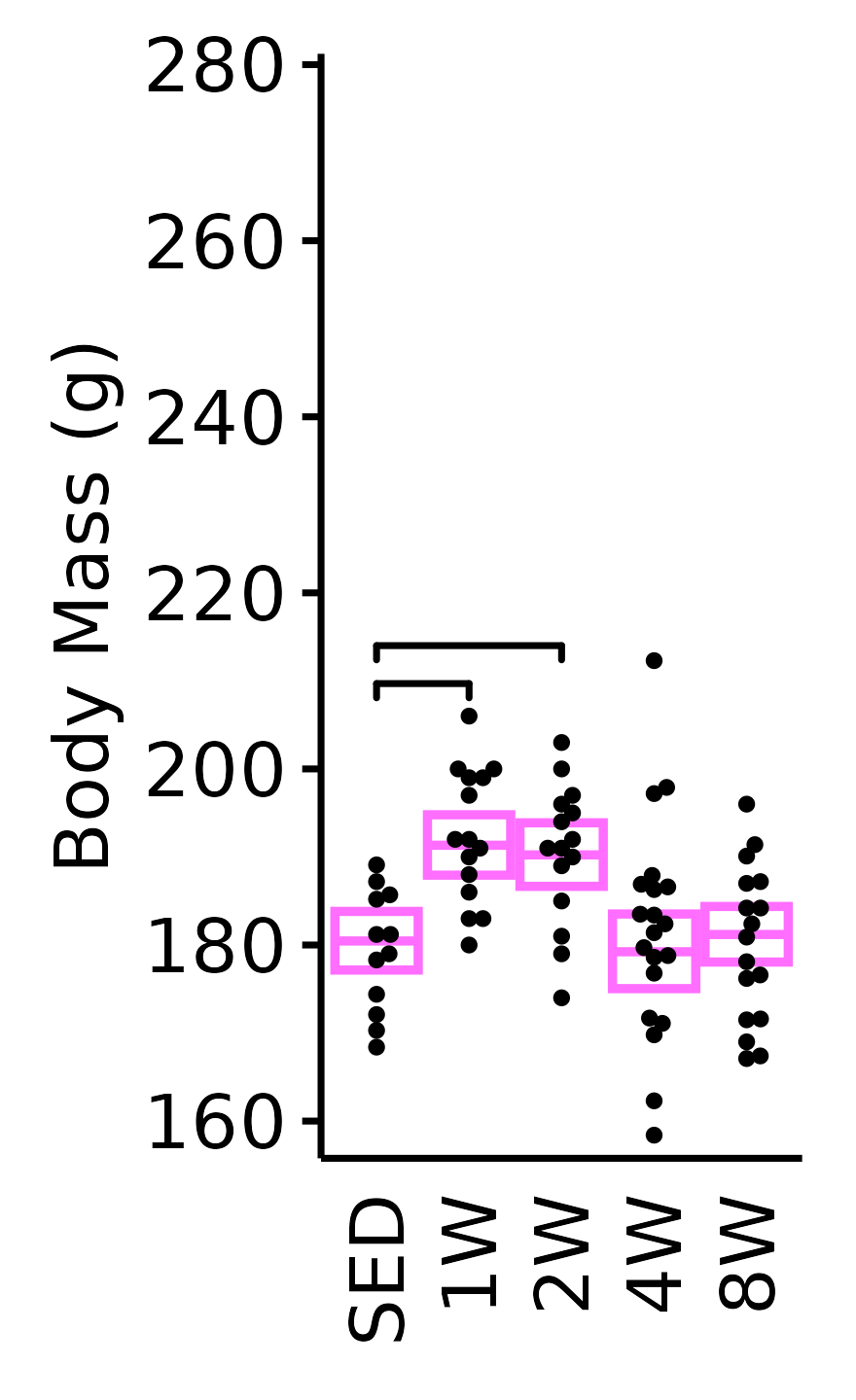
6M Male
plot_baseline(x = NMR,
              response = "pre_body_mass",
              conf = filter(conf_df, response == "NMR Body Mass"),
              stats = filter(BASELINE_STATS, response == "NMR Body Mass"),
              sex = "Male", age = "6M", y_position = 420,
              step_increase = 0.06) +
  scale_y_continuous(name = "Body Mass (g)",
                     breaks = seq(270, 470, 40),
                     expand = expansion(mult = 1e-2)) +
  coord_cartesian(ylim = c(270, 470), clip = "off") +
  theme(plot.margin = unit(c(12, 5, 5, 5), units = "pt"))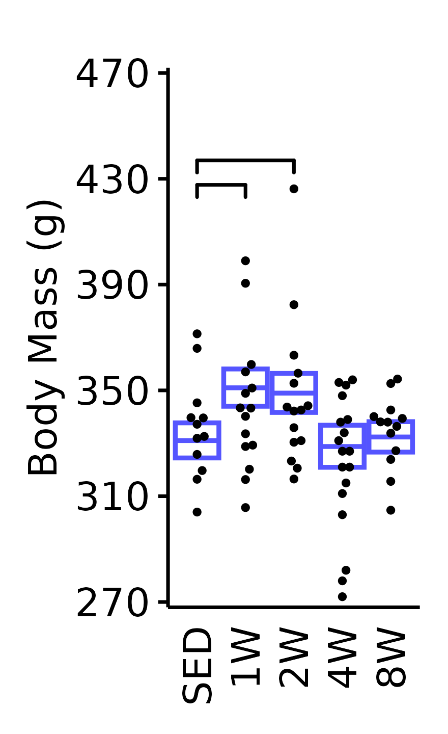
18M Female
plot_baseline(x = NMR, response = "pre_body_mass",
              conf = filter(conf_df, response == "NMR Body Mass"),
              stats = filter(BASELINE_STATS, response == "NMR Body Mass"),
              sex = "Female", age = "18M", y_position = 265) +
  scale_y_continuous(name = "Body Mass (g)",
                     breaks = seq(160, 280, 20),
                     expand = expansion(mult = 1e-2)) +
  coord_cartesian(ylim = c(157, 280), clip = "off") +
  theme(plot.margin = unit(c(5, 5, 5, 5), units = "pt"))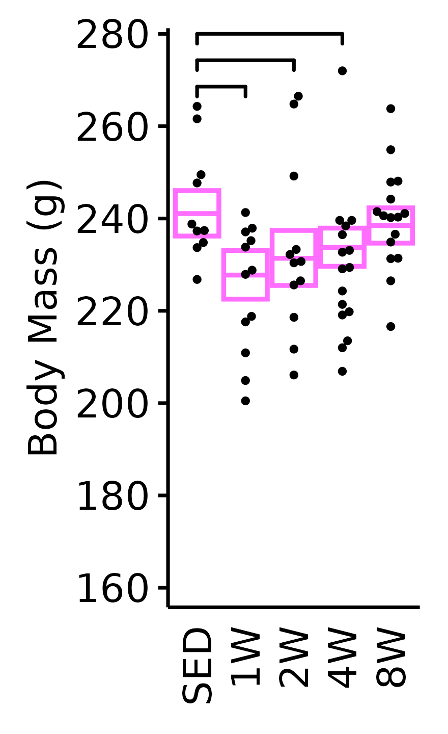
18M Male
plot_baseline(x = NMR, response = "pre_body_mass",
              conf = filter(conf_df, response == "NMR Body Mass"),
              stats = filter(BASELINE_STATS, response == "NMR Body Mass"),
              sex = "Male", age = "18M", y_position = 472) +
  scale_y_continuous(name = "Body Mass (g)",
                     breaks = seq(270, 470, 40),
                     expand = expansion(mult = 1e-2)) +
  coord_cartesian(ylim = c(270, 470), clip = "off") +
  theme(plot.margin = unit(c(12, 5, 5, 5), units = "pt"))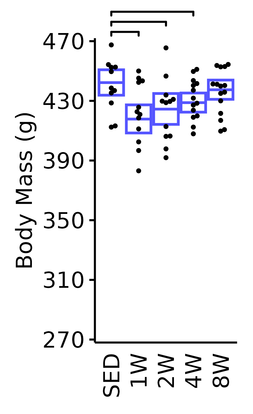
NMR Lean Mass
Lean mass (g) recorded via NMR.
6M Female
plot_baseline(x = NMR, response = "pre_lean",
              conf = filter(conf_df, response == "NMR Lean Mass"),
              stats = filter(BASELINE_STATS, response == "NMR Lean Mass"),
              sex = "Female", age = "6M", y_position = 123) +
  scale_y_continuous(name = "NMR Lean Mass (g)",
                     breaks = seq(90, 150, 10),
                     expand = expansion(mult = 1e-2)) +
  coord_cartesian(ylim = c(90, 150), clip = "off") +
  theme(plot.margin = unit(c(12, 3, 3, 3), units = "pt"))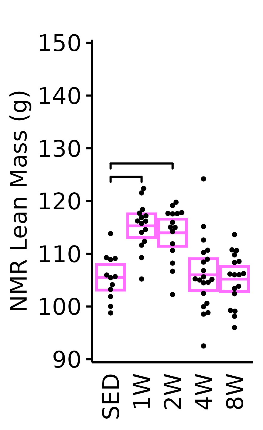
6M Male
plot_baseline(x = NMR, response = "pre_lean",
              conf = filter(conf_df, response == "NMR Lean Mass"),
              stats = filter(BASELINE_STATS, response == "NMR Lean Mass"),
              sex = "Male", age = "6M") +
  scale_y_continuous(name = "NMR Lean Mass (g)",
                     breaks = seq(150, 240, 20),
                     expand = expansion(mult = 1e-2)) +
  coord_cartesian(ylim = c(150, 240), clip = "off") +
  theme(plot.margin = unit(c(10, 3, 3, 3), units = "pt"))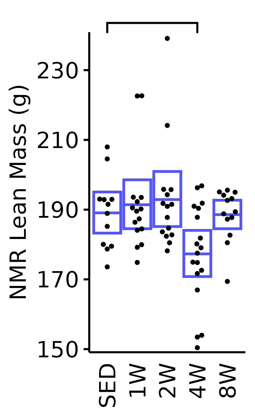
18M Female
plot_baseline(x = NMR, response = "pre_lean",
              conf = filter(conf_df, response == "NMR Lean Mass"),
              stats = filter(BASELINE_STATS, response == "NMR Lean Mass"),
              sex = "Female", age = "18M", y_position = 146) +
  scale_y_continuous(name = "NMR Lean Mass (g)",
                     breaks = seq(90, 150, 10),
                     expand = expansion(mult = 1e-2)) +
  coord_cartesian(ylim = c(90, 150), clip = "off") +
  theme(plot.margin = unit(c(12, 3, 3, 3), units = "pt"))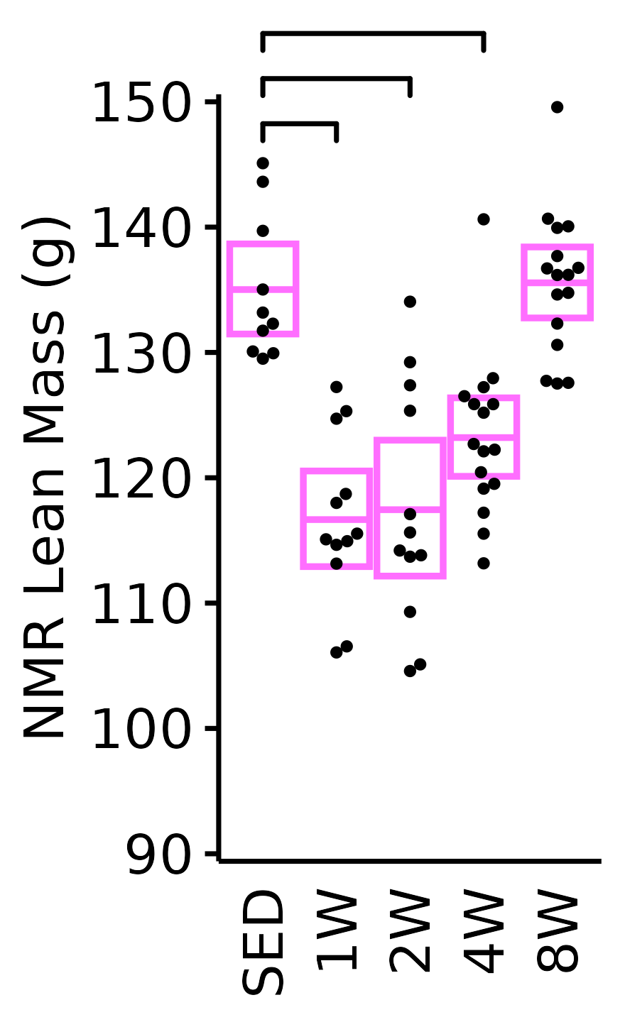
18M Male
plot_baseline(x = NMR, response = "pre_lean",
              conf = filter(conf_df, response == "NMR Lean Mass"),
              stats = filter(BASELINE_STATS, response == "NMR Lean Mass"),
              sex = "Male", age = "18M") +
  scale_y_continuous(name = "NMR Lean Mass (g)",
                     breaks = seq(150, 240, 20),
                     expand = expansion(mult = 1e-2)) +
  coord_cartesian(ylim = c(150, 240), clip = "off") +
  theme(plot.margin = unit(c(10, 3, 3, 3), units = "pt"))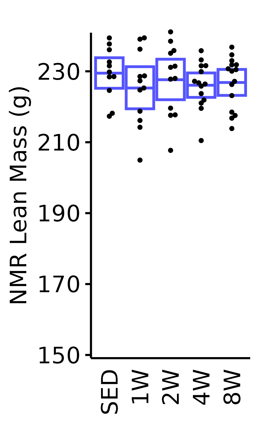
NMR Fat Mass
Fat mass (g) recorded via NMR.
6M Female
plot_baseline(x = NMR, response = "pre_fat",
              conf = filter(conf_df, response == "NMR Fat Mass"),
              stats = filter(BASELINE_STATS, response == "NMR Fat Mass"),
              sex = "Female", age = "6M", y_position = 33) +
  scale_y_continuous(name = "NMR Fat Mass (g)",
                     breaks = seq(10, 60, 10),
                     expand = expansion(mult = 1e-2)) +
  coord_cartesian(ylim = c(10, 62), clip = "off") +
  theme(plot.margin = unit(c(6, 3, 3, 3), units = "pt"))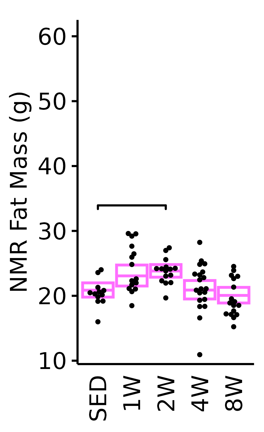
6M Male
plot_baseline(x = NMR, response = "pre_fat",
              conf = filter(conf_df, response == "NMR Fat Mass"),
              stats = filter(BASELINE_STATS, response == "NMR Fat Mass"),
              sex = "Male", age = "6M") +
  scale_y_continuous(name = "NMR Fat Mass (g)",
                     breaks = seq(40, 100, 10),
                     expand = expansion(mult = 1e-2)) +
  coord_cartesian(ylim = c(35, 100), clip = "off") +
  theme(plot.margin = unit(c(10, 3, 3, 3), units = "pt"))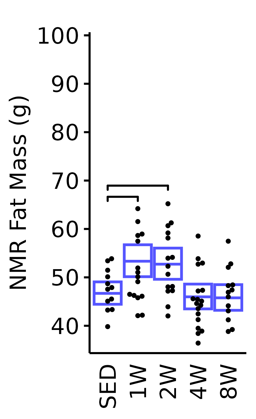
18M Female
plot_baseline(x = NMR, response = "pre_fat",
              conf = filter(conf_df, response == "NMR Fat Mass"),
              stats = filter(BASELINE_STATS, response == "NMR Fat Mass"),
              sex = "Female", age = "18M", y_position = 57) +
  scale_y_continuous(name = "NMR Fat Mass (g)",
                     breaks = seq(10, 60, 10),
                     expand = expansion(mult = 1e-2)) +
  coord_cartesian(ylim = c(10, 62), clip = "off") +
  theme(plot.margin = unit(c(6, 3, 3, 3), units = "pt"))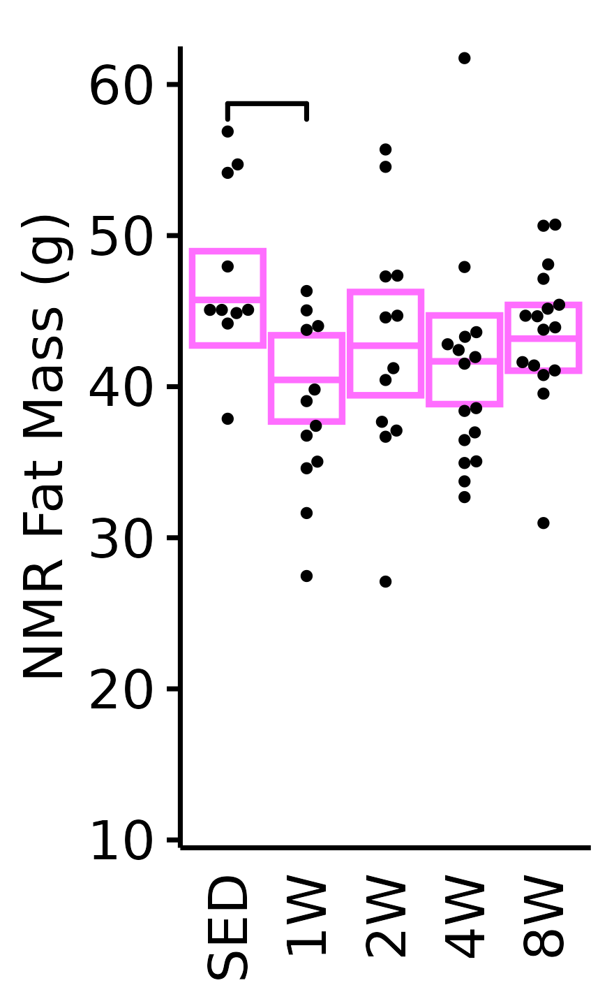
18M Male
plot_baseline(x = NMR, response = "pre_fat",
              conf = filter(conf_df, response == "NMR Fat Mass"),
              stats = filter(BASELINE_STATS, response == "NMR Fat Mass"),
              sex = "Male", age = "18M") +
  scale_y_continuous(name = "NMR Fat Mass (g)",
                     breaks = seq(40, 100, 10),
                     expand = expansion(mult = 1e-2)) +
  coord_cartesian(ylim = c(35, 100), clip = "off") +
  theme(plot.margin = unit(c(10, 3, 3, 3), units = "pt"))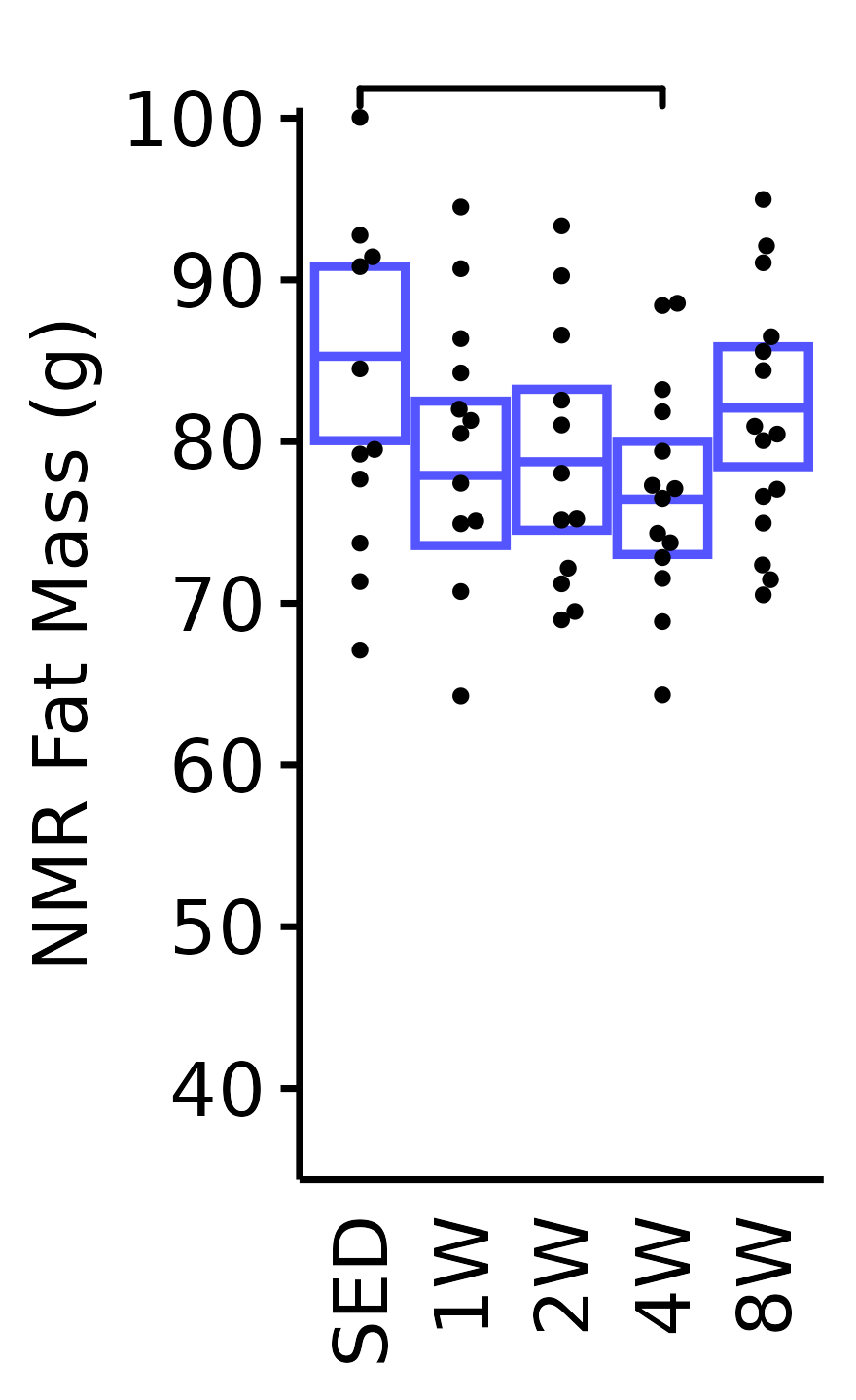
NMR % Lean
Lean mass (g) recorded via NMR divided by the body mass (g) recorded on the same day and then multiplied by 100%.
6M Female
plot_baseline(x = NMR, response = "pre_lean_pct",
              conf = filter(conf_df, response == "NMR % Lean"),
              stats = filter(BASELINE_STATS, response == "NMR % Lean"),
              sex = "Female", age = "6M") +
  scale_y_continuous(name = "NMR % Lean Mass",
                     breaks = seq(48, 64, 4),
                     expand = expansion(mult = 1e-2)) +
  coord_cartesian(ylim = c(48, 64), clip = "off") +
  theme(plot.margin = unit(c(3, 3, 3, 3), units = "pt"))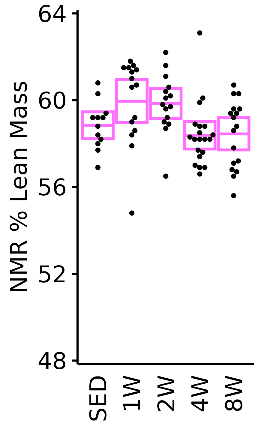
6M Male
plot_baseline(x = NMR, response = "pre_lean_pct",
              conf = filter(conf_df, response == "NMR % Lean"),
              stats = filter(BASELINE_STATS, response == "NMR % Lean"),
              sex = "Male", age = "6M") +
  scale_y_continuous(name = "NMR % Lean Mass",
                     breaks = seq(50, 58, 2),
                     expand = expansion(mult = 1e-2)) +
  coord_cartesian(ylim = c(49.7, 58.5), clip = "off") +
  theme(plot.margin = unit(c(12, 3, 3, 3), units = "pt"))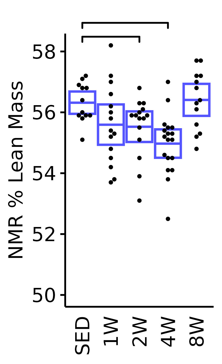
18M Female
plot_baseline(x = NMR, response = "pre_lean_pct",
              conf = filter(conf_df, response == "NMR % Lean"),
              stats = filter(BASELINE_STATS, response == "NMR % Lean"),
              sex = "Female", age = "18M", y_position = 57.4) +
  labs(y  = "NMR % Lean Mass") +
  scale_y_continuous(name = "NMR % Lean Mass",
                     breaks = seq(48, 64, 4),
                     expand = expansion(mult = 1e-2)) +
  coord_cartesian(ylim = c(48, 64), clip = "off") +
  theme(plot.margin = unit(c(3, 3, 3, 3), units = "pt"))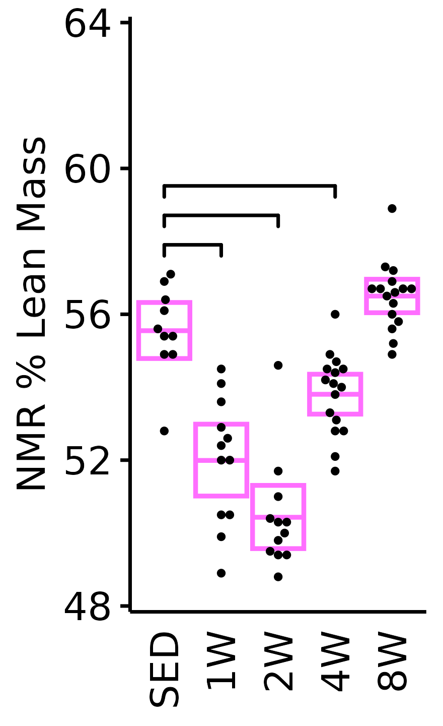
18M Male
plot_baseline(x = NMR, response = "pre_lean_pct",
              conf = filter(conf_df, response == "NMR % Lean"),
              stats = filter(BASELINE_STATS, response == "NMR % Lean"),
              sex = "Male", age = "18M", y_position = 55.7) +
  scale_y_continuous(name = "NMR % Lean Mass",
                     breaks = seq(50, 58, 2),
                     expand = expansion(mult = 1e-2)) +
  coord_cartesian(ylim = c(49.7, 58.5), clip = "off") +
  theme(plot.margin = unit(c(12, 3, 3, 3), units = "pt"))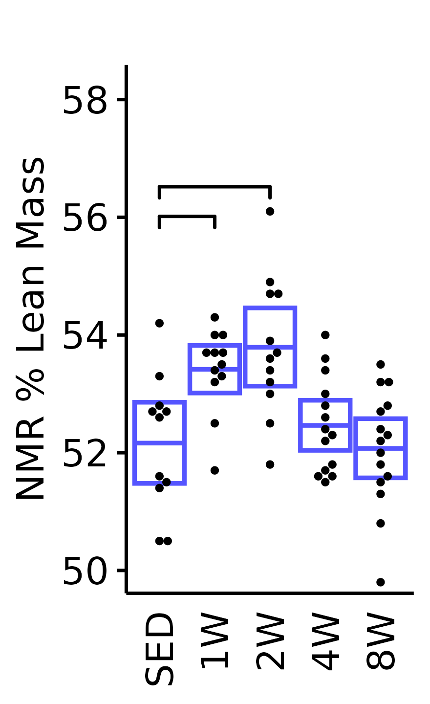
NMR % Fat
Fat mass (g) recorded via NMR divided by the body mass (g) recorded on the same day and then multiplied by 100%.
6M Female
plot_baseline(x = NMR, response = "pre_fat_pct",
              conf = filter(conf_df, response == "NMR % Fat"),
              stats = filter(BASELINE_STATS, response == "NMR % Fat"),
              sex = "Female", age = "6M") +
  scale_y_continuous(name = "NMR % Fat Mass",
                     breaks = seq(8, 24, 4),
                     expand = expansion(mult = 1e-2)) +
  coord_cartesian(ylim = c(6.7, 24), clip = "off") +
  theme(plot.margin = unit(c(5, 3, 3, 3), units = "pt"))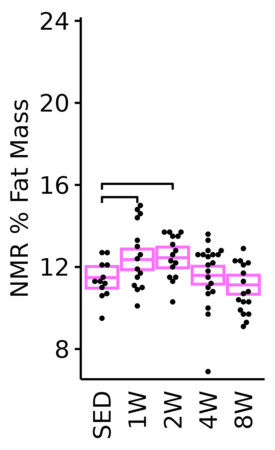
6M Male
plot_baseline(x = NMR, response = "pre_fat_pct",
              conf = filter(conf_df, response == "NMR % Fat"),
              stats = filter(BASELINE_STATS, response == "NMR % Fat"),
              sex = "Male", age = "6M") +
  scale_y_continuous(name = "NMR % Fat Mass",
                     breaks = seq(12, 22, 2),
                     expand = expansion(mult = 1e-2)) +
  coord_cartesian(ylim = c(11.3, 22), clip = "off") +
  theme(plot.margin = unit(c(3, 3, 3, 3), units = "pt"))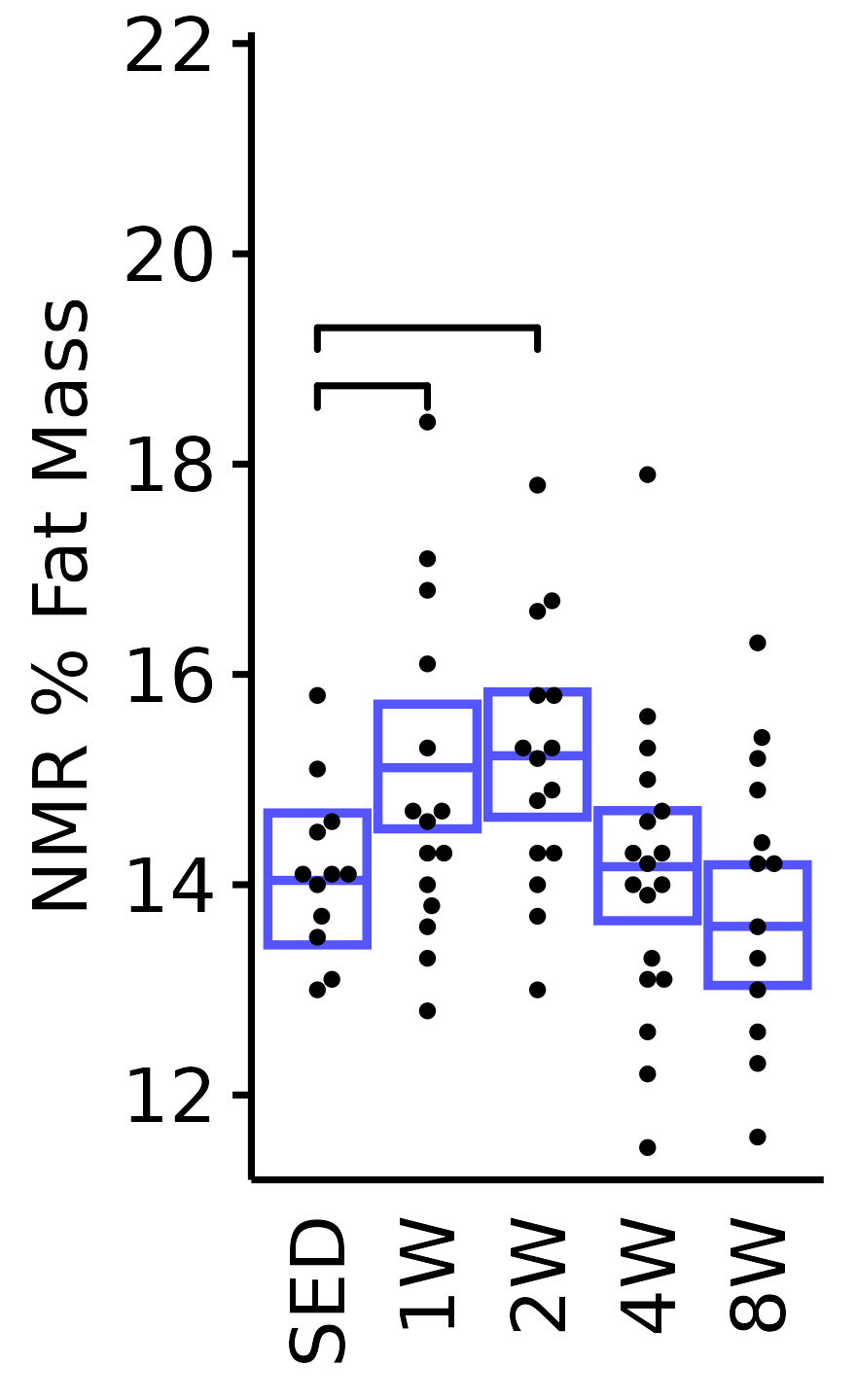
18M Female
plot_baseline(x = NMR, response = "pre_fat_pct",
              conf = filter(conf_df, response == "NMR % Fat"),
              stats = filter(BASELINE_STATS, response == "NMR % Fat"),
              sex = "Female", age = "18M", y_position = 23) +
  scale_y_continuous(name = "NMR % Fat Mass",
                     breaks = seq(8, 24, 4),
                     expand = expansion(mult = 1e-2)) +
  coord_cartesian(ylim = c(6.7, 24), clip = "off") +
  theme(plot.margin = unit(c(5, 3, 3, 3), units = "pt"))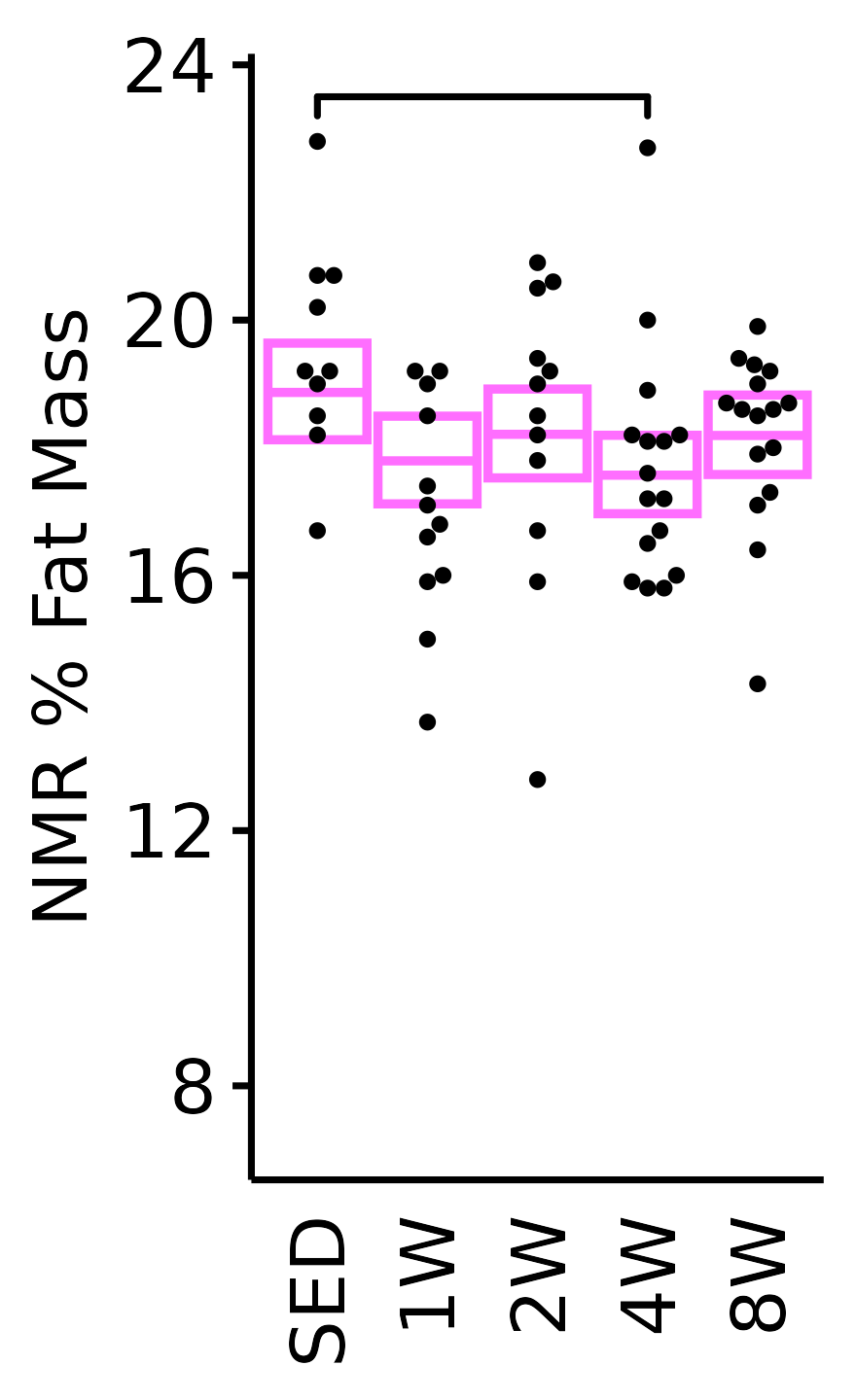
18M Male
plot_baseline(x = NMR, response = "pre_fat_pct",
              conf = filter(conf_df, response == "NMR % Fat"),
              stats = filter(BASELINE_STATS, response == "NMR % Fat"),
              sex = "Male", age = "18M") +
  scale_y_continuous(name = "NMR % Fat Mass",
                     breaks = seq(12, 22, 2),
                     expand = expansion(mult = 1e-2)) +
  coord_cartesian(ylim = c(11.3, 22), clip = "off") +
  theme(plot.margin = unit(c(3, 3, 3, 3), units = "pt"))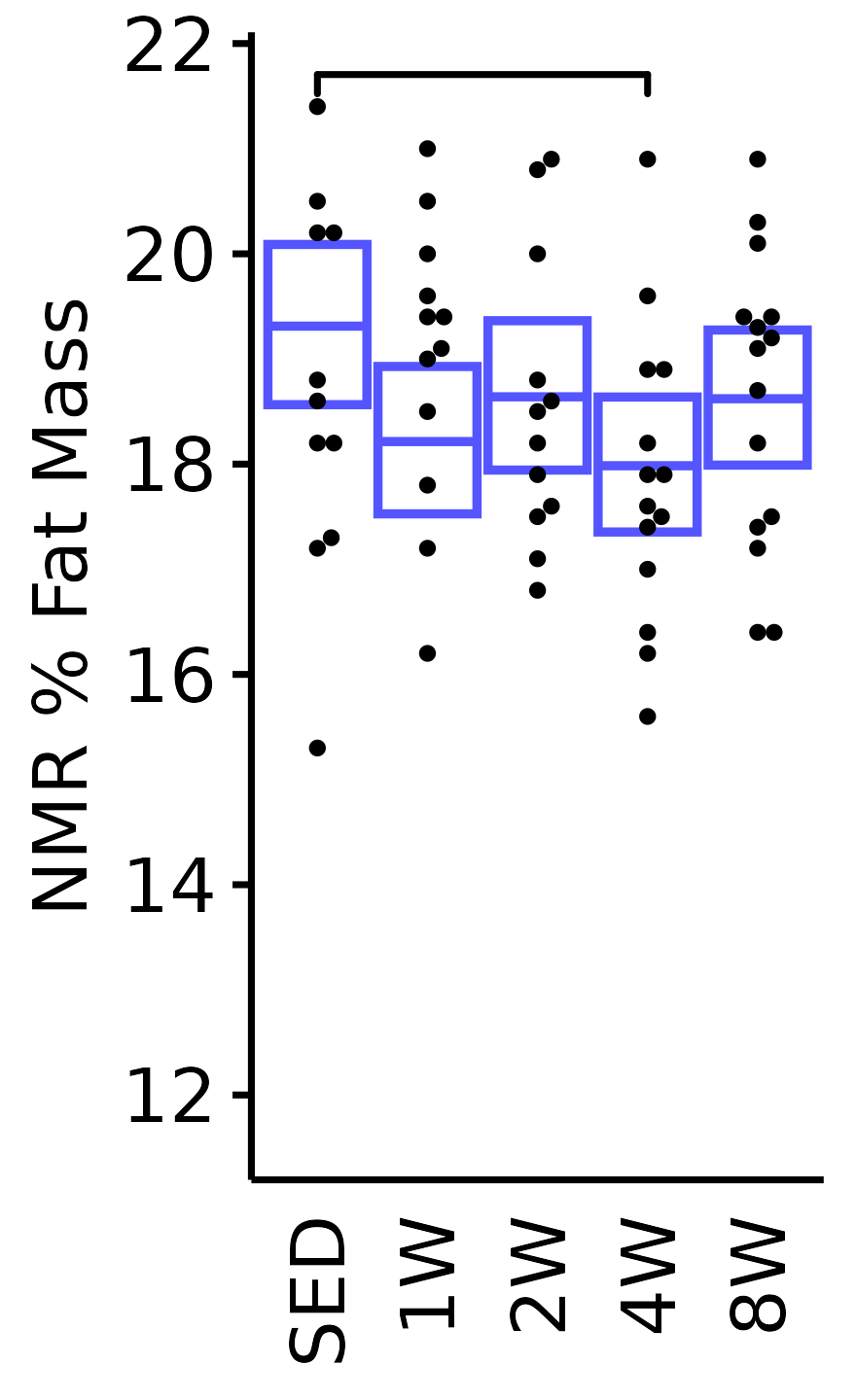
Absolute VO\(_2\)max
Absolute VO\(_2\)max is calculated by multiplying relative VO\(_2\)max (\(mL \cdot kg^{-1} \cdot min^{-1}\)) by body mass (kg).
6M Female
plot_baseline(x = VO2MAX, response = "pre_vo2max_ml_min",
              conf = filter(conf_df, response == "Absolute VO2max"),
              stats = filter(BASELINE_STATS, response == "Absolute VO2max"),
              sex = "Female", age = "6M") +
  scale_y_continuous(name = TeX("VO$_2$max (mL/min)"),
                     breaks = seq(11, 16, 1),
                     expand = expansion(mult = 1e-2)) +
  coord_cartesian(ylim = c(10.8, 16), clip = "off") +
  theme(plot.margin = unit(c(3, 3, 3, 3), units = "pt"))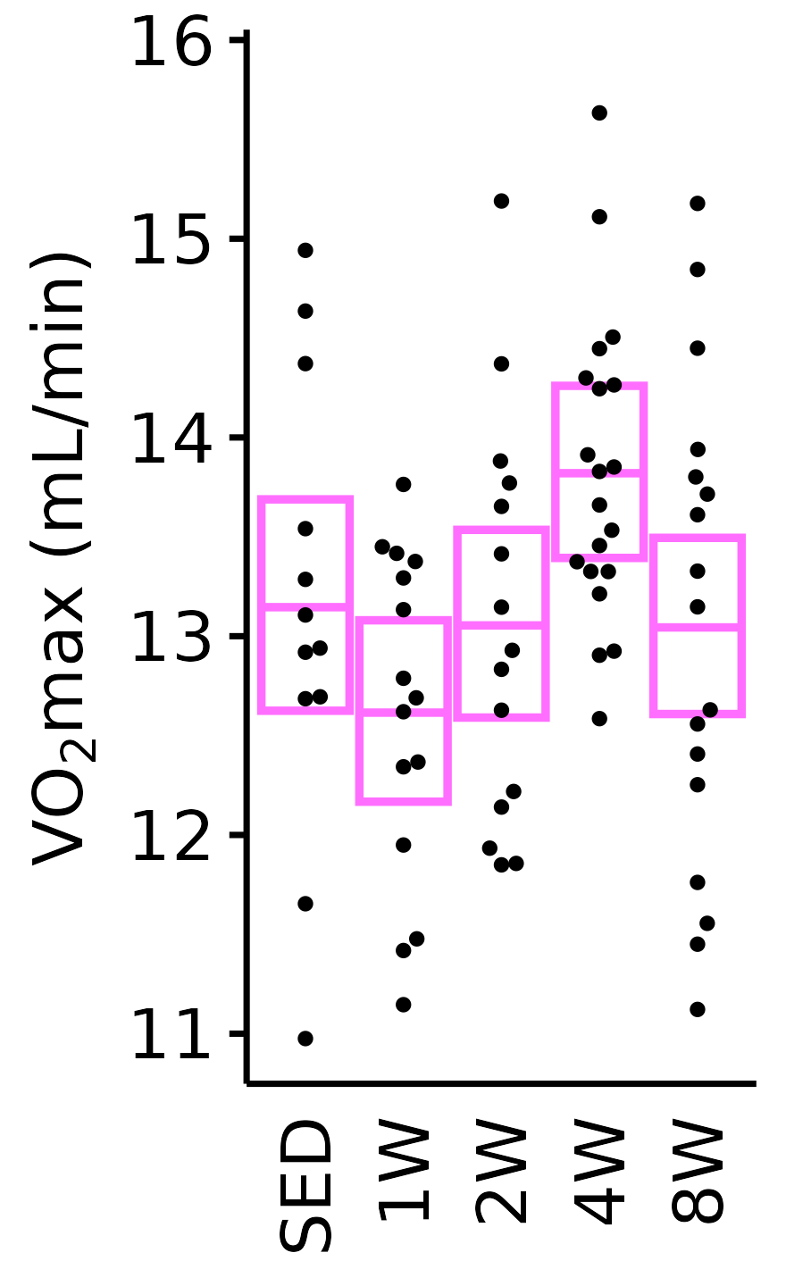
6M Male
plot_baseline(x = VO2MAX, response = "pre_vo2max_ml_min",
              conf = filter(conf_df, response == "Absolute VO2max"),
              stats = filter(BASELINE_STATS, response == "Absolute VO2max"),
              sex = "Male", age = "6M", y_position = 26) +
  scale_y_continuous(name = TeX("VO$_2$max (mL/min)"),
                     breaks = seq(18, 30, 2),
                     expand = expansion(mult = 1e-2)) +
  coord_cartesian(ylim = c(17.5, 30), clip = "off") +
  theme(plot.margin = unit(c(3, 3, 3, 3), units = "pt"))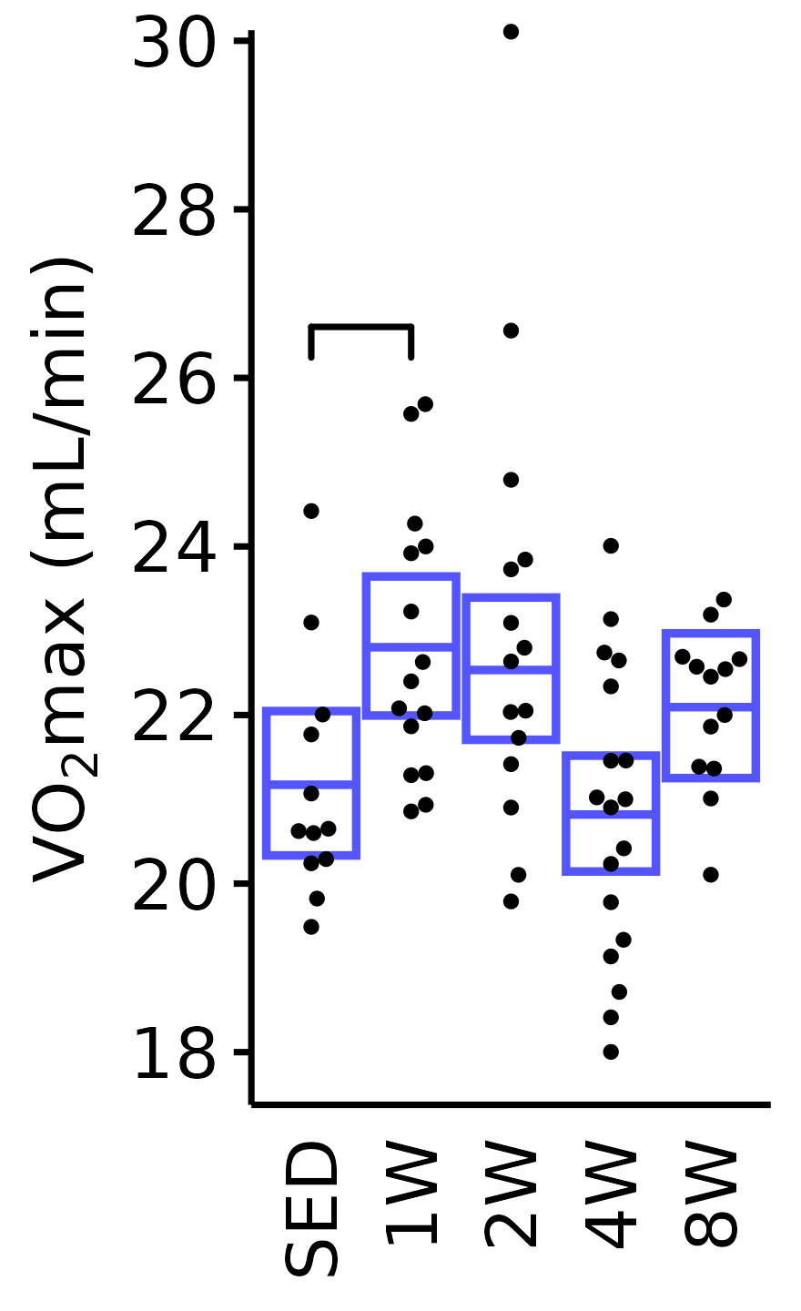
18M Female
plot_baseline(x = VO2MAX, response = "pre_vo2max_ml_min",
              conf = filter(conf_df, response == "Absolute VO2max"),
              stats = filter(BASELINE_STATS, response == "Absolute VO2max"),
              sex = "Female", age = "18M") +
  scale_y_continuous(name = TeX("VO$_2$max (mL/min)"),
                     breaks = seq(11, 16, 1),
                     expand = expansion(mult = 1e-2)) +
  coord_cartesian(ylim = c(10.8, 16), clip = "off") +
  theme(plot.margin = unit(c(3, 3, 3, 3), units = "pt"))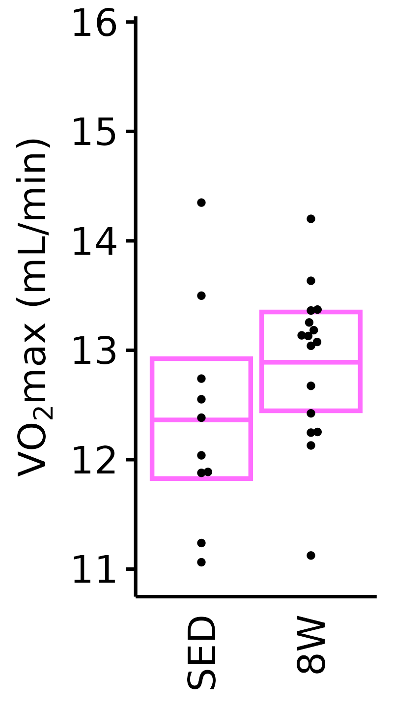
18M Male
plot_baseline(x = VO2MAX, response = "pre_vo2max_ml_min",
              conf = filter(conf_df, response == "Absolute VO2max"),
              stats = filter(BASELINE_STATS, response == "Absolute VO2max"),
              sex = "Male", age = "18M") +
  scale_y_continuous(name = TeX("VO$_2$max (mL/min)"),
                     breaks = seq(18, 30, 2),
                     expand = expansion(mult = 1e-2)) +
  coord_cartesian(ylim = c(17.5, 30), clip = "off") +
  theme(plot.margin = unit(c(3, 3, 3, 3), units = "pt"))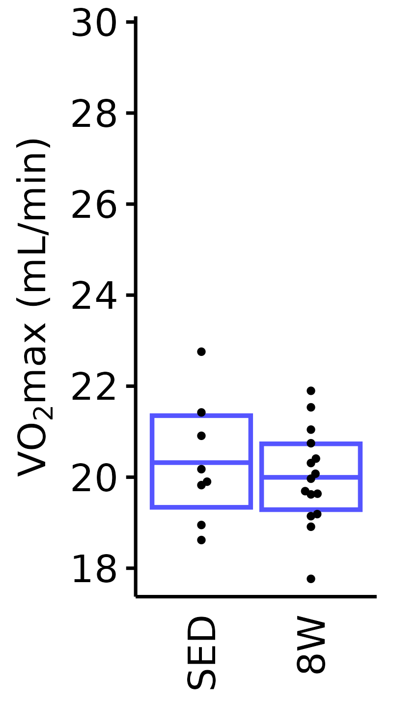
Relative VO\(_2\)max
Relative VO\(_2\)max (mL/kg body mass/min).
6M Female
plot_baseline(x = VO2MAX, response = "pre_vo2max_ml_kg_min",
              conf = filter(conf_df, response == "Relative VO2max"),
              stats = filter(BASELINE_STATS, response == "Relative VO2max"),
              sex = "Female", age = "6M") +
  scale_y_continuous(name = TeX("VO$_2$max (mL/kg/min)"),
                     breaks = seq(45, 85, 10),
                     expand = expansion(mult = 1e-2)) +
  coord_cartesian(ylim = c(45, 85), clip = "off") +
  theme(plot.margin = unit(c(3, 3, 3, 3), units = "pt"))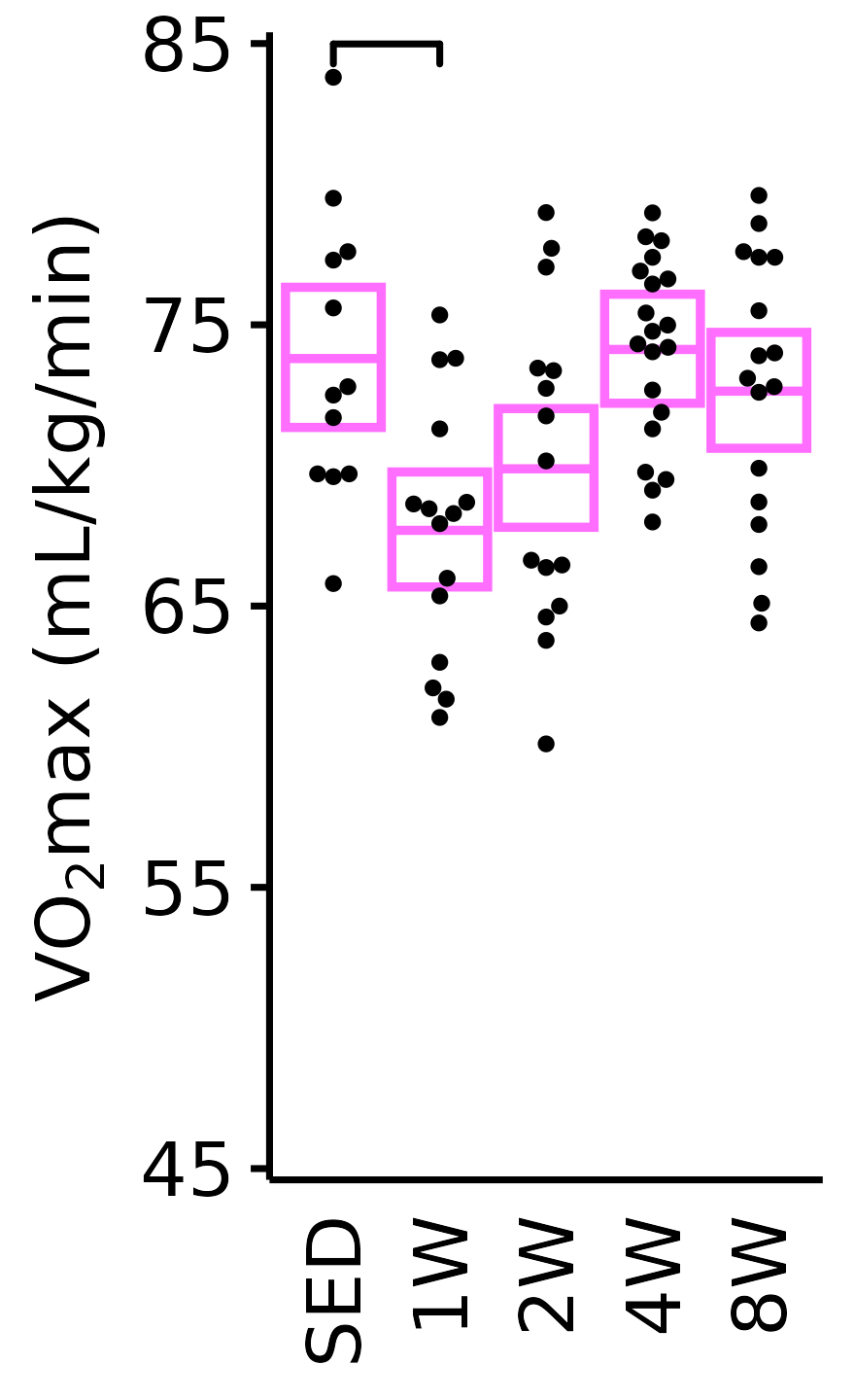
6M Male
plot_baseline(x = VO2MAX, response = "pre_vo2max_ml_kg_min",
              conf = filter(conf_df, response == "Relative VO2max"),
              stats = filter(BASELINE_STATS, response == "Relative VO2max"),
              sex = "Male", age = "6M") +
  scale_y_continuous(name = TeX("VO$_2$max (mL/kg/min)"),
                     breaks = seq(40, 80, 10),
                     expand = expansion(mult = 1e-2)) +
  coord_cartesian(ylim = c(40, 80), clip = "off") +
  theme(plot.margin = unit(c(3, 3, 3, 3), units = "pt"))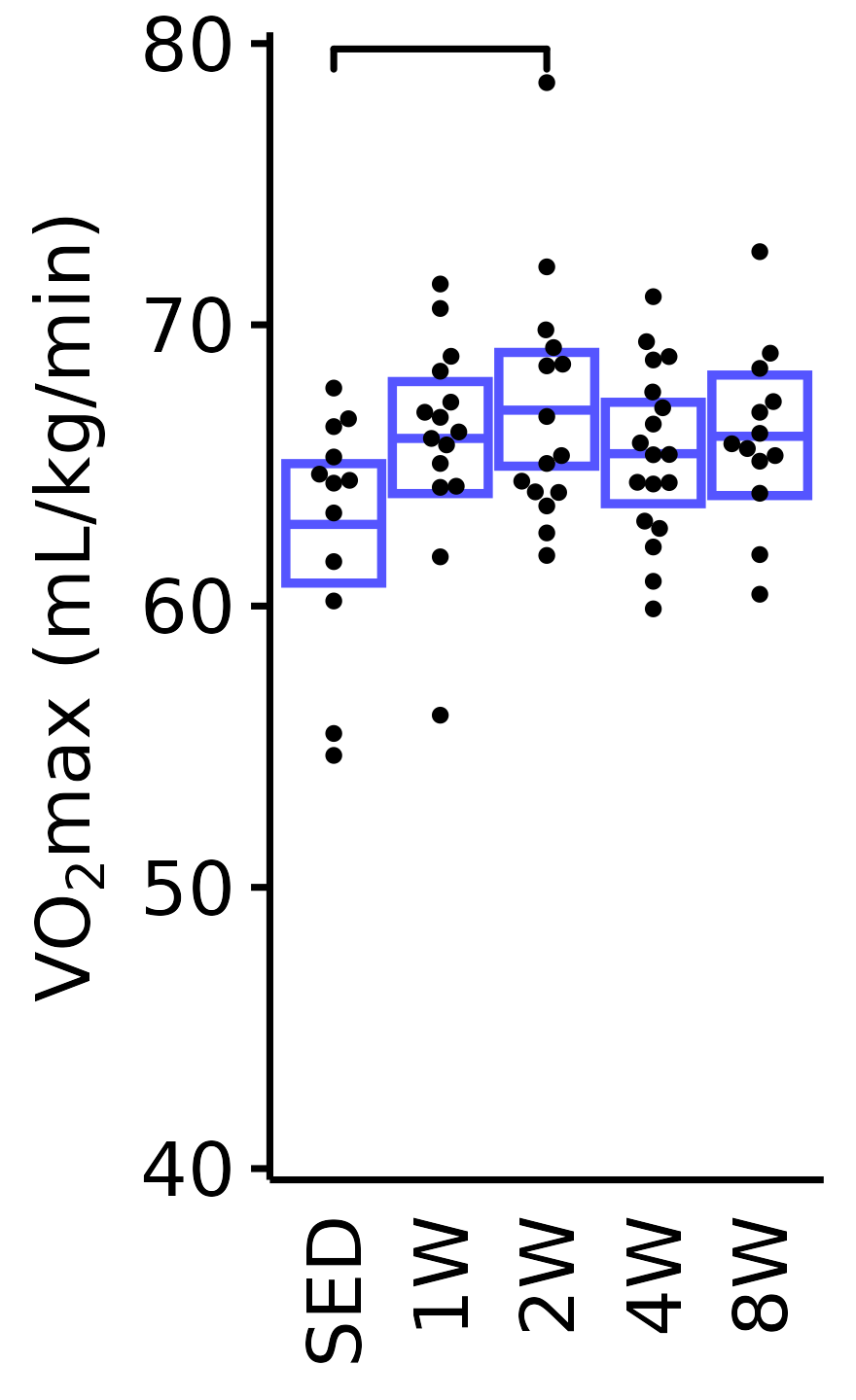
18M Female
plot_baseline(x = VO2MAX, response = "pre_vo2max_ml_kg_min",
              conf = filter(conf_df, response == "Relative VO2max"),
              stats = filter(BASELINE_STATS, response == "Relative VO2max"),
              sex = "Female", age = "18M", y_position = 66) +
  scale_y_continuous(name = TeX("VO$_2$max (mL/kg/min)"),
                     breaks = seq(45, 85, 10),
                     expand = expansion(mult = 1e-2)) +
  coord_cartesian(ylim = c(45, 85), clip = "off") +
  theme(plot.margin = unit(c(3, 3, 3, 3), units = "pt"))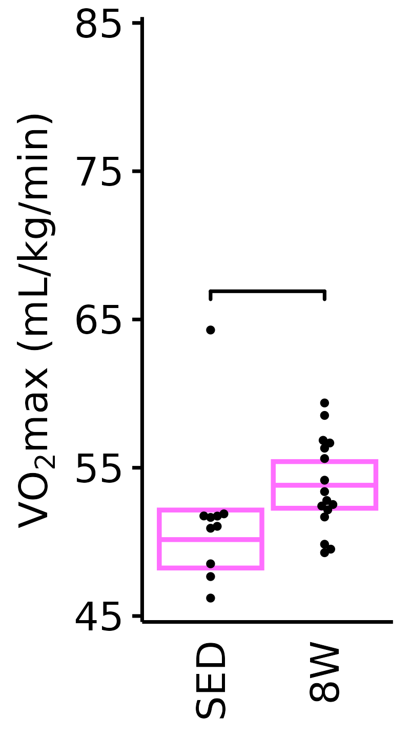
18M Male
plot_baseline(x = VO2MAX, response = "pre_vo2max_ml_kg_min",
              conf = filter(conf_df, response == "Relative VO2max"),
              stats = filter(BASELINE_STATS, response == "Relative VO2max"),
              sex = "Male", age = "18M") +
  scale_y_continuous(name = TeX("VO$_2$max (mL/kg/min)"),
                     breaks = seq(40, 80, 10),
                     expand = expansion(mult = 1e-2)) +
  coord_cartesian(ylim = c(40, 80), clip = "off") +
  theme(plot.margin = unit(c(3, 3, 3, 3), units = "pt"))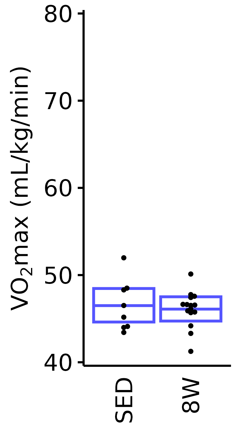
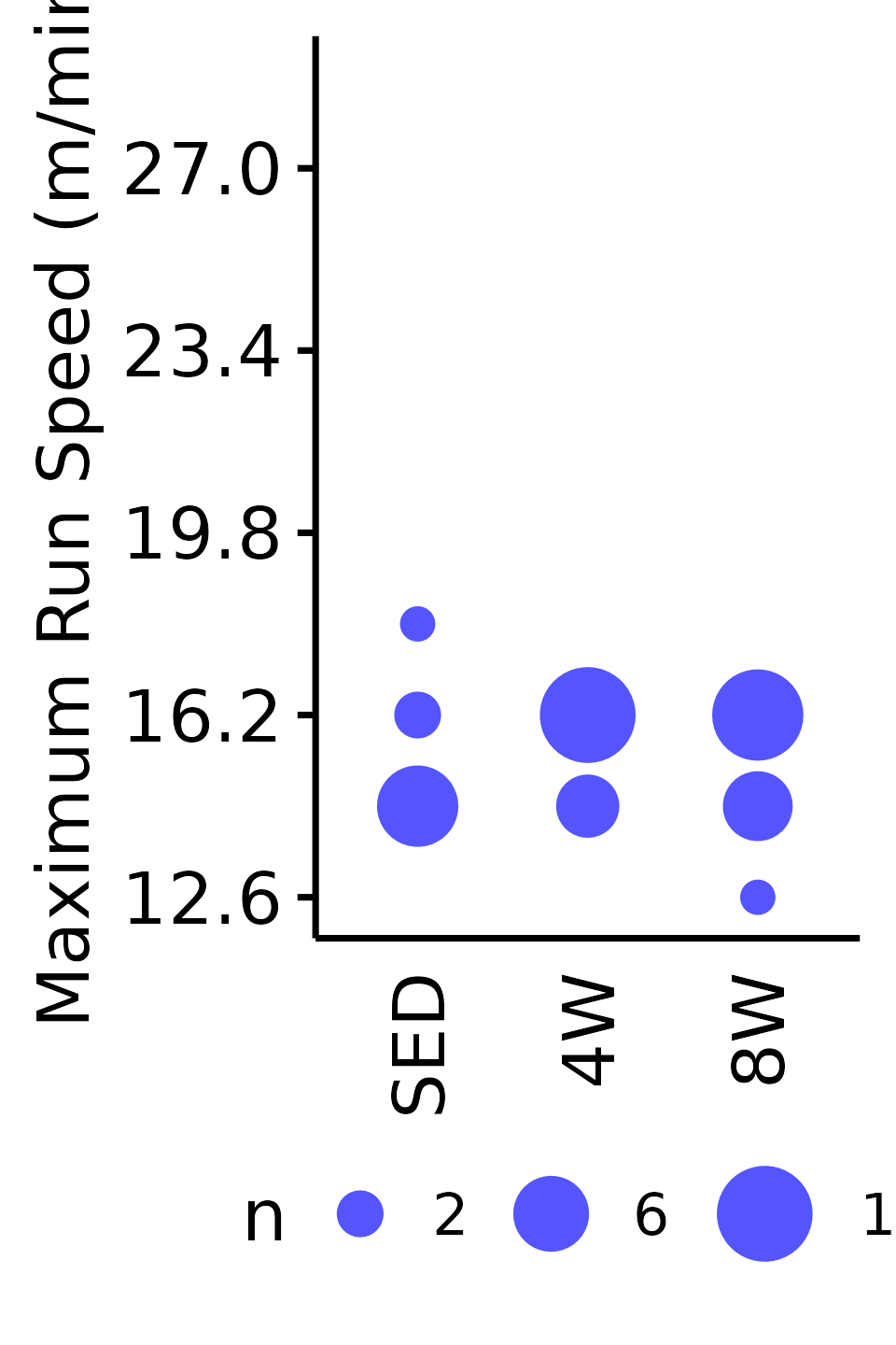
Maximum Run Speed
The maximum running speed reached by each rat (m/min). Speed was increased by 1.8 m/min increments, so the non-parametric Wilcoxon Rank Sum test was used. Rather than plotting the individual points, since they can only take on a few different values, we will instead count the number of samples that take on a particular value in each group and scale the points accordingly.
# Custom theme for maximum run speed plots
t1 <- theme(text = element_text(size = 7, color = "black"),
            line = element_line(linewidth = 0.3, color = "black"),
            axis.ticks = element_line(linewidth = 0.3, color = "black"),
            panel.grid = element_blank(),
            panel.border = element_blank(),
            axis.ticks.x = element_blank(),
            axis.text = element_text(size = 7,
                                     color = "black"),
            axis.text.x = element_text(size = 7, angle = 90, hjust = 1,
                                       vjust = 0.5),
            axis.title = element_text(size = 7, margin = margin(),
                                      color = "black"),
            axis.line = element_line(linewidth = 0.3),
            strip.background = element_blank(),
            strip.text = element_blank(),
            panel.spacing = unit(-1, "pt"),
            plot.title = element_text(size = 7, color = "black"),
            plot.subtitle = element_text(size = 7, color = "black"),
            legend.position = "bottom",
            legend.direction = "horizontal",
            legend.title.align = 0.5,
            legend.key.size = unit(7, "pt"),
            legend.box.spacing = unit(0, "pt"),
            legend.box.margin = margin(t = 0, b = 0, unit = "pt"),
            strip.placement = "outside"
)
6M Female
VO2MAX %>%
  filter(sex == "Female", age == "6M") %>%
  count(age, sex, group, pre_speed_max) %>%
  ggplot(aes(x = group, y = pre_speed_max, size = n)) +
  geom_point(shape = 16, color = "#ff6eff") +
  scale_size_area(max_size = 4, breaks = seq(2, 10, 4)) +
  scale_y_continuous(name = "Maximum Run Speed (m/min)",
                     breaks = seq(12.6, 36, 3.6),
                     limits = c(12.6, 28.8)) +
  labs(x = NULL) +
  theme_bw(base_size = 7) +
  t1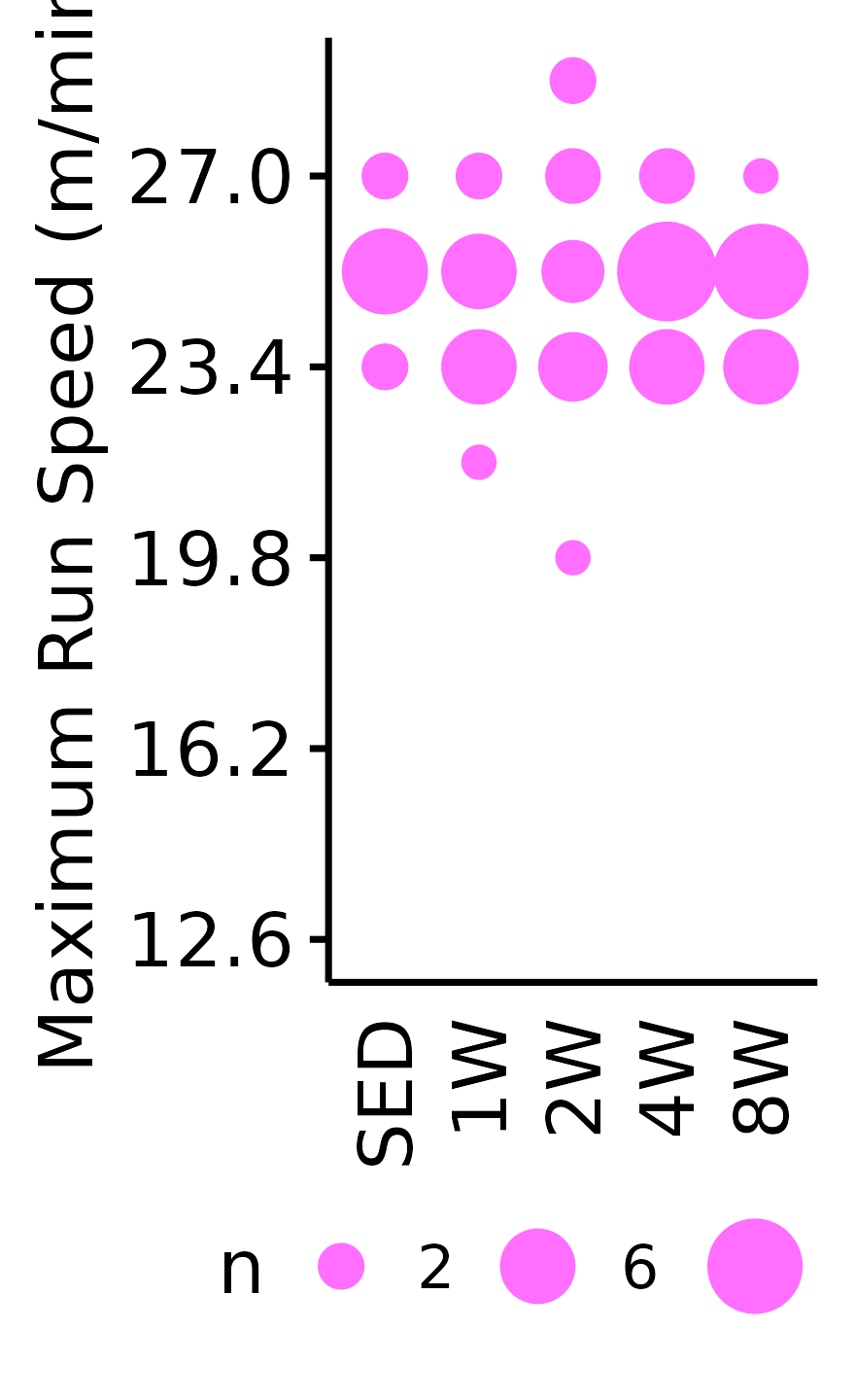
6M Male
VO2MAX %>%
  filter(sex == "Male", age == "6M") %>%
  count(age, sex, group, pre_speed_max) %>%
  ggplot(aes(x = group, y = pre_speed_max, size = n)) +
  geom_point(shape = 16, color = "#5555ff") +
  ggpubr::stat_pvalue_manual(
    data = data.frame(y.position = c(23.4, 25.2) + 1.2,
                      group1 = rep("SED", 2),
                      group2 = c("1W", "2W"),
                      label = rep("", 2))
  ) +
  scale_size_area(max_size = 4, breaks = seq(2, 10, 4)) +
  scale_y_continuous(name = "Maximum Run Speed (m/min)",
                     breaks = seq(12.6, 36, 3.6),
                     limits = c(12.6, 28.8)) +
  labs(x = NULL) +
  theme_bw(base_size = 6) +
  t1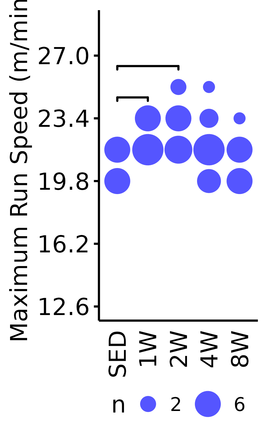
18M Female
VO2MAX %>%
  filter(sex == "Female", age == "18M") %>%
  count(age, sex, group, pre_speed_max) %>%
  ggplot(aes(x = group, y = pre_speed_max, size = n)) +
  geom_point(shape = 16, color = "#ff6eff") +
  scale_size_area(max_size = 4, breaks = seq(2, 10, 4)) +
  scale_y_continuous(name = "Maximum Run Speed (m/min)",
                     breaks = seq(12.6, 36, 3.6),
                     limits = c(12.6, 28.8)) +
  labs(x = NULL) +
  theme_bw(base_size = 7) +
  t1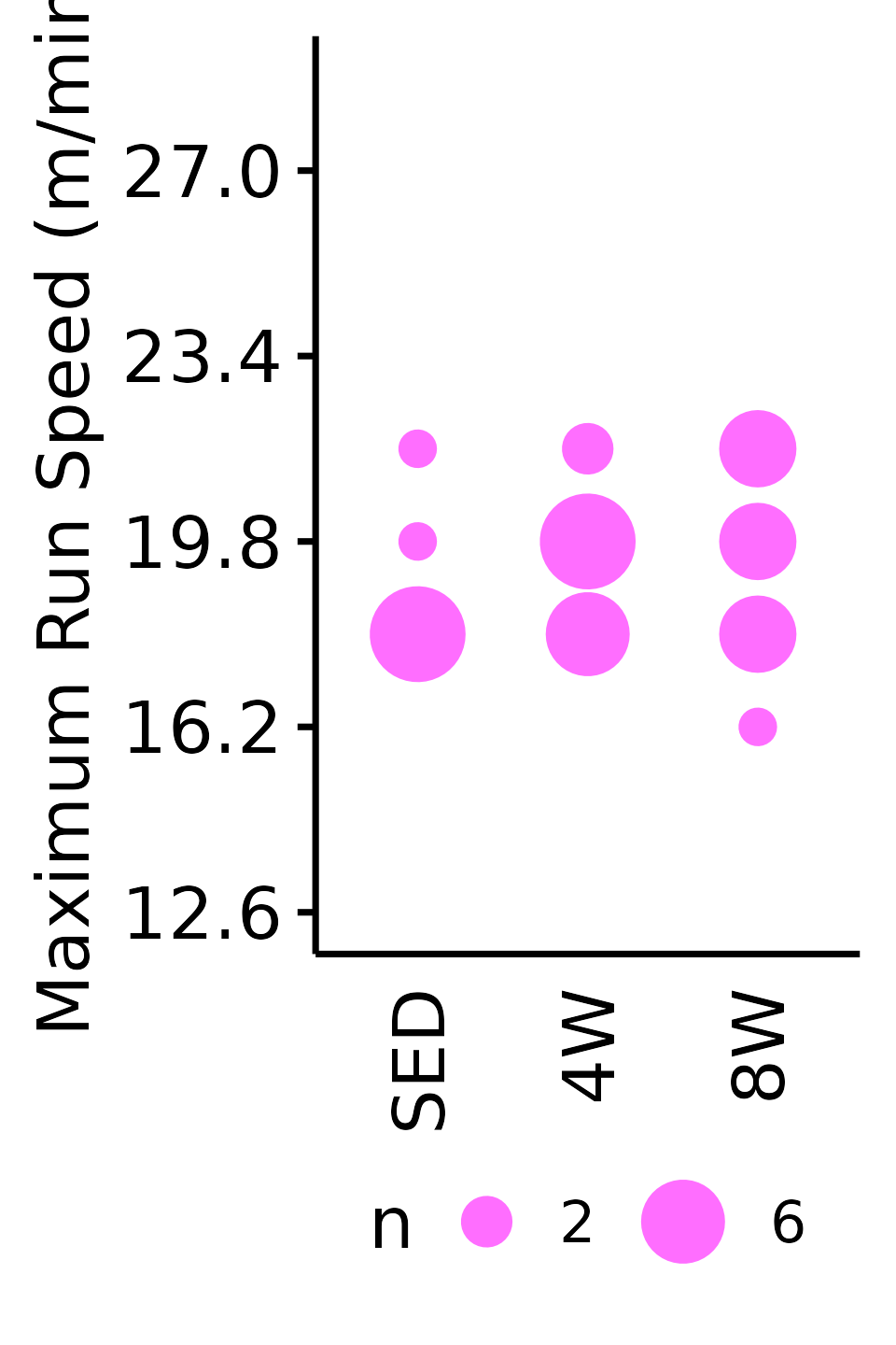
18M Male
VO2MAX %>%
  filter(sex == "Male", age == "18M") %>%
  count(age, sex, group, pre_speed_max) %>%
  ggplot(aes(x = group, y = pre_speed_max, size = n)) +
  geom_point(shape = 16, color = "#5555ff", na.rm = TRUE) +
  scale_size_area(max_size = 4, breaks = seq(2, 10, 4)) +
  scale_y_continuous(name = "Maximum Run Speed (m/min)",
                     breaks = seq(12.6, 36, 3.6),
                     limits = c(12.6, 28.8)) +
  labs(x = NULL) +
  theme_bw(base_size = 7) +
  t1